The Researcher's Complete Guide to Statistical Test Selection
The Researcher's Complete Guide to Statistical Test Selection
1. From Confusion to Clarity: A Decision-Tree Approach to Hypothesis Testing
"Statistics is the grammar of science." — Karl Pearson
But what good is grammar if you don't know which words to use?
If you've ever stared at your data wondering whether to run a t-test or Mann-Whitney, ANOVA or Kruskal-Wallis, Pearson or Spearman—you're not alone. This guide exists because statistical test selection shouldn't require a PhD in mathematics. It should be a decision tree you can follow.
What makes this guide different:
- Decision trees first: Navigate to your test, don't memorize everything
- Engineer-friendly math: Formulas that make intuitive sense
- "Don't use this when" sections: Knowing what NOT to do is half the battle
- Real examples: From actual research scenarios
- Visual explanations: Geometry over algebra wherever possible
Table of Contents
- Chapter 1: The Foundation — What You Must Know First
- Chapter 2: Understanding Distributions — The Shape of Your Data
- Chapter 3: The Master Decision Tree — Your Navigation System
- Chapter 4: Assumption Testing — The Gates You Must Pass
- Chapter 5: Comparing Groups — The Core Tests
- Chapter 6: Relationships Between Variables — Correlation Tests
- Chapter 7: Effect Size — The Forgotten Hero
- Chapter 8: Categorical Data Analysis
- Chapter 9: Advanced Techniques
- Chapter 10: Bayesian Alternatives — The Other Paradigm
- Chapter 11: Statistical Sins Researchers Commit
- Chapter 12: Quick Reference & Cheat Sheets
Chapter 1: The Foundation — What You Must Know First
Before we dive into test selection, let's establish the fundamental concepts that everything else builds upon. Think of this chapter as learning the alphabet before writing sentences.
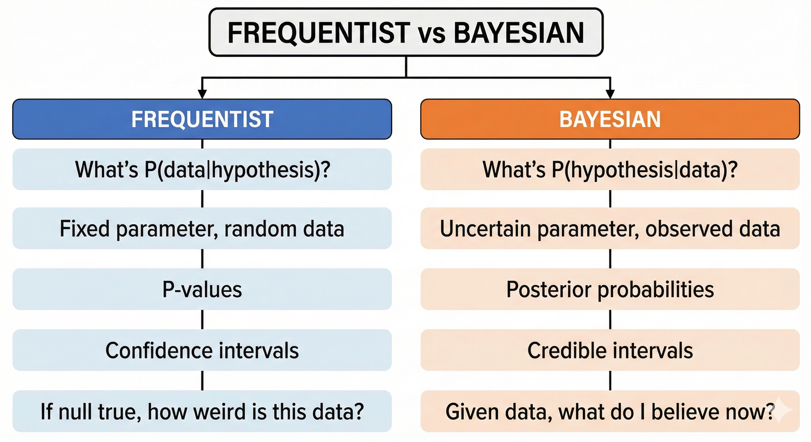
2. 1.1 The Two Tribes: Frequentist vs. Bayesian
Statistical inference has two major philosophical camps. Understanding which camp your chosen test belongs to helps you interpret results correctly.
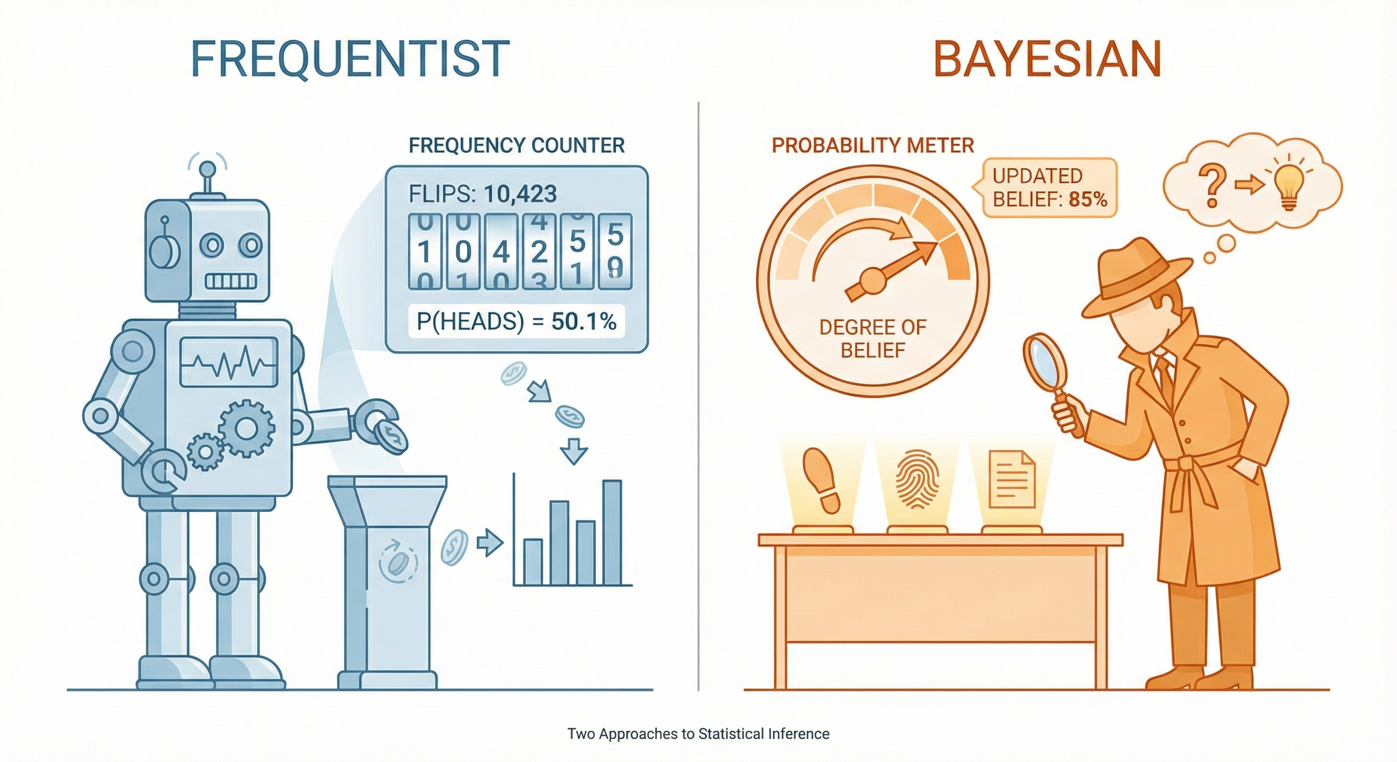
2.1. Frequentist Approach (The Dominant Paradigm)
Core belief: Probability represents long-run frequencies of events.
Imagine flipping a coin 10,000 times. The frequentist says: "The probability of heads is the proportion of heads I'd get if I repeated this infinitely."
Key characteristics:
- Parameters (like population mean) are fixed but unknown
- Data is random
- We calculate: "What's the probability of seeing this data IF the null hypothesis is true?"
- Results in p-values and confidence intervals
Analogy: A frequentist is like a factory quality inspector who tests 1000 light bulbs to estimate the defect rate. The true defect rate is fixed; they're trying to estimate it through repeated sampling.
2.2. Bayesian Approach (The Rising Alternative)
Core belief: Probability represents degrees of belief or certainty.
Key characteristics:
- Parameters have probability distributions (they're uncertain)
- We update prior beliefs with data to get posterior beliefs
- We calculate: "What's the probability of this hypothesis GIVEN the data I observed?"
- Results in posterior distributions and credible intervals
Analogy: A Bayesian is like a detective who starts with hunches (priors) and updates their beliefs as evidence comes in. Their certainty about who committed the crime changes with each clue.
3. 1.2 The P-Value: Most Misunderstood Statistic in Science
3.1. What a P-Value Actually Is
Definition: The p-value is the probability of obtaining results at least as extreme as the observed results, assuming the null hypothesis is true.
Let's break this down with an analogy:
The Courtroom Analogy:
- Null hypothesis (H₀): The defendant is innocent
- Alternative hypothesis (H₁): The defendant is guilty
- Evidence: Your data
- P-value: How surprising would this evidence be IF the defendant were truly innocent?
A small p-value (say, 0.001) means: "If the defendant were innocent, there's only a 0.1% chance we'd see evidence this damning. This evidence is very surprising under the innocence assumption."
3.2. The Mathematical Formula
Where:
- T is the test statistic (a number summarizing your data)
- t_observed is the actual value you calculated from your sample
- H₀ is the null hypothesis
Geometric Interpretation:
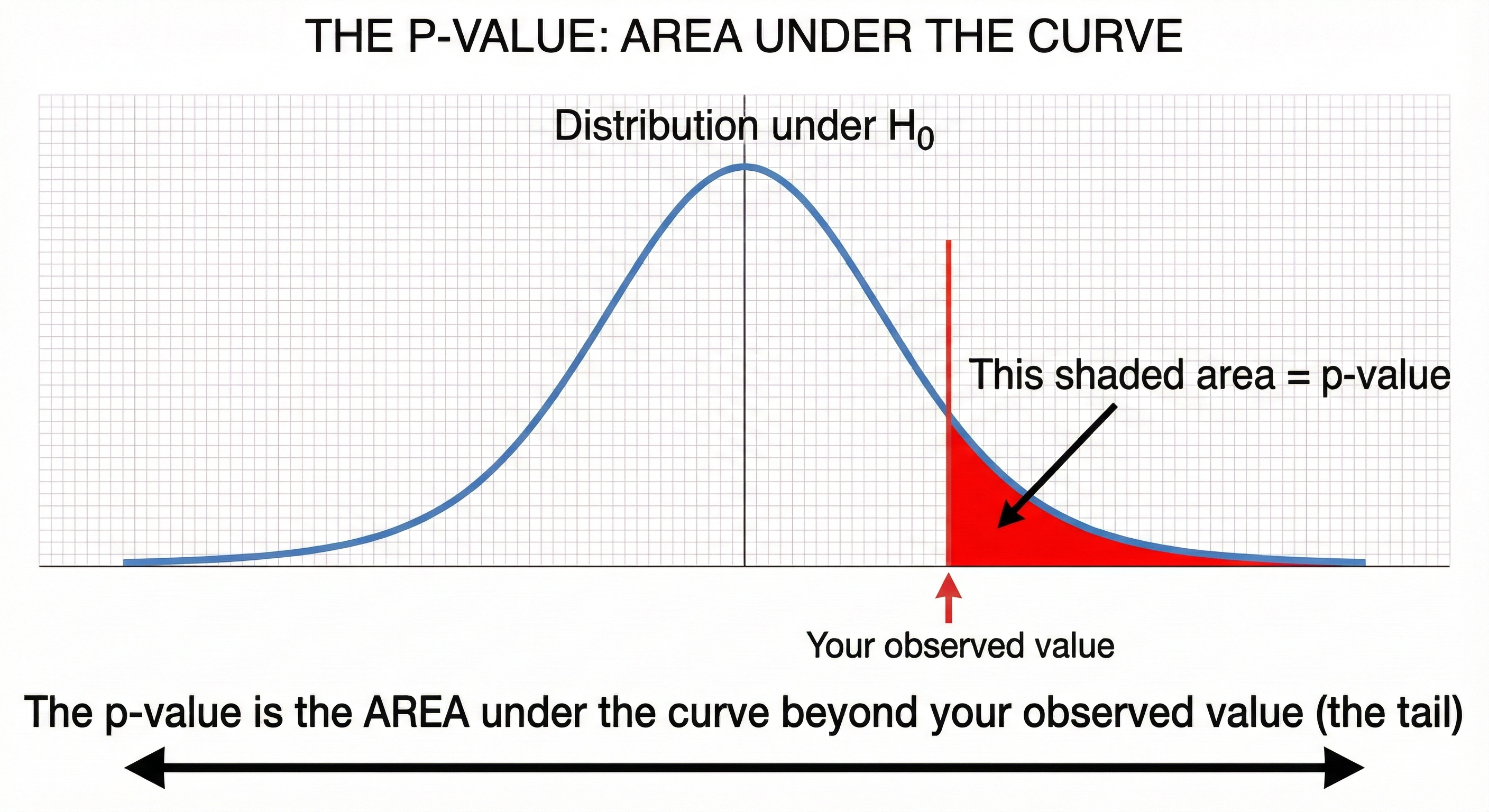
3.3. What P-Values Are NOT
| Common Misconception | Reality |
|---|---|
| "P-value is the probability the null hypothesis is true" | NO. It's P(data|H₀), not P(H₀|data) |
| "P = 0.05 means 5% chance results are due to chance" | NO. It means IF H₀ is true, 5% of experiments would show results this extreme |
| "P < 0.05 means my effect is important/large" | NO. Statistical significance ≠ practical significance |
| "P = 0.06 is 'trending toward significance'" | NO. Either your threshold is 0.05 or it isn't. There's no "trending." |
| "Non-significant p means no effect exists" | NO. Absence of evidence ≠ evidence of absence |
3.4. Computing P-Values: The General Process
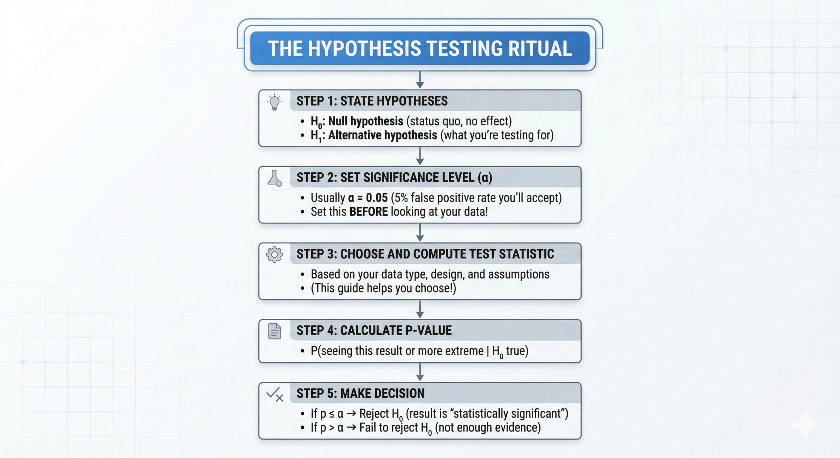
- State your hypotheses (H₀ and H₁)
- Choose a test statistic (t, F, χ², Z, etc.)
- Calculate the test statistic from your data
- Find the probability of getting a value this extreme or more extreme under H₀
- This requires knowing the distribution of your test statistic under H₀
- Usually involves looking up tables or using software
Example Calculation:
Suppose you're testing if a new interface design reduces task completion time. Your null hypothesis is "no difference."
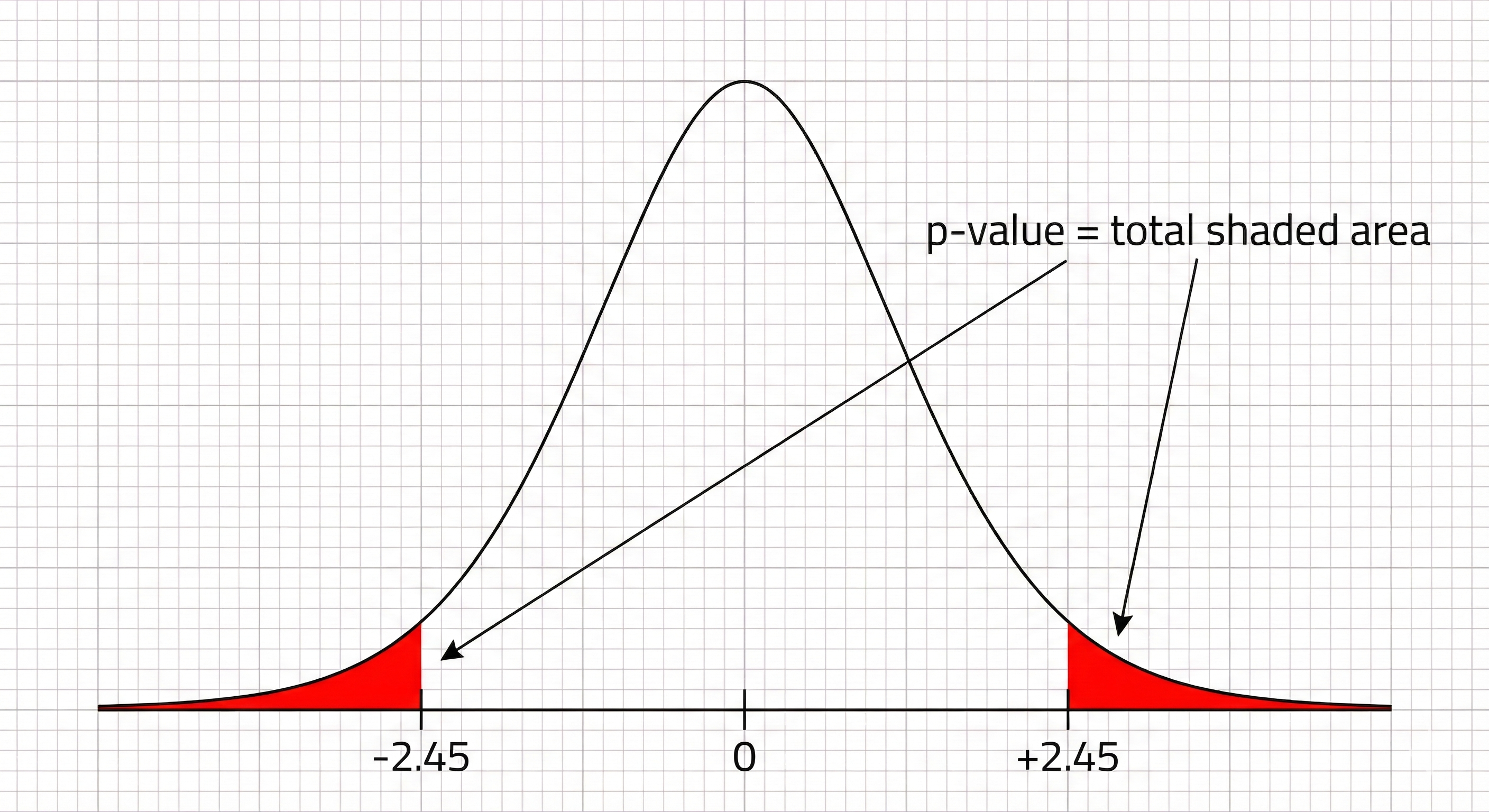
You collect data and calculate a t-statistic of 2.45 with 28 degrees of freedom.
The p-value = P(|T| ≥ 2.45 | H₀ is true)
Looking at a t-distribution with df=28, the area in both tails beyond ±2.45 is approximately 0.021.
So p ≈ 0.021, meaning: "If there truly were no difference, we'd see a result this extreme only about 2.1% of the time."
4. 1.3 Hypothesis Testing: The Scientific Ritual
4.1. The Five-Step Framework
Every statistical test follows this ritual:
4.2. Type I and Type II Errors: The Two Ways to Be Wrong
| H₀ is Actually True | H₀ is Actually False | |
|---|---|---|
| Reject H₀ | Type I Error (α) False Positive "Crying wolf" | Correct! True Positive (Power = 1-β) |
| Fail to Reject H₀ | Correct! True Negative | Type II Error (β) False Negative "Missing the wolf" |
Memorable analogy:
- Type I Error: Convicting an innocent person (false alarm)
- Type II Error: Letting a guilty person go free (missed detection)
The Trade-off: Reducing Type I errors (being more conservative) increases Type II errors, and vice versa. You can't minimize both simultaneously with fixed sample size.
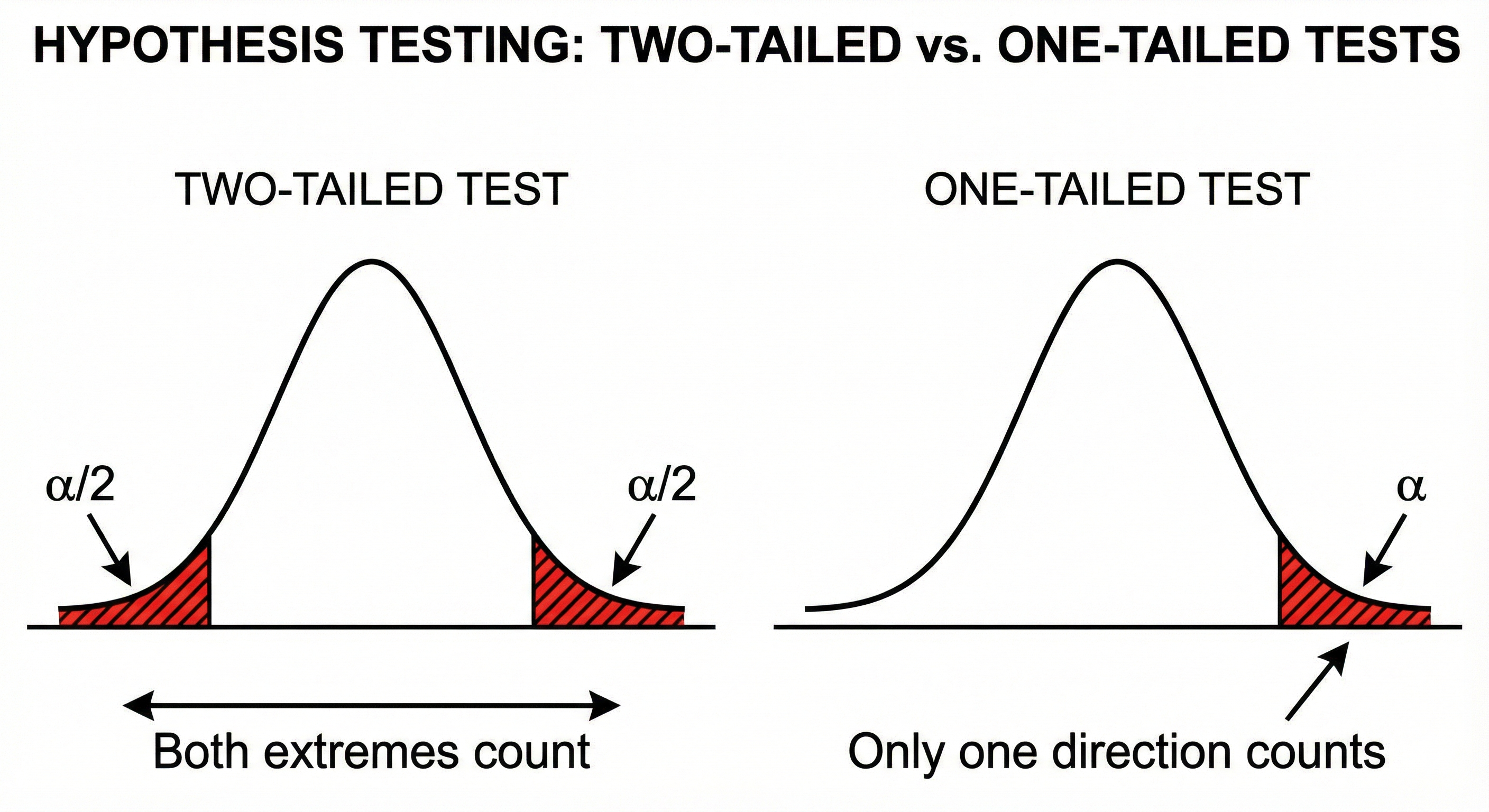
4.3. One-Tailed vs. Two-Tailed Tests
Two-tailed test: You're testing for ANY difference (could be higher OR lower)
- H₁: μ₁ ≠ μ₂
- P-value considers both tails of the distribution
- Use when you have no directional prediction
One-tailed test: You're testing for a SPECIFIC direction
- H₁: μ₁ > μ₂ (or μ₁ < μ₂)
- P-value considers only one tail
- Use when you have a strong directional hypothesis BEFORE collecting data
⚠️ Don't use this when: You decide to use one-tailed AFTER seeing your data goes in a particular direction. This is p-hacking!
5. 1.4 Statistical Power: Your Test's Ability to Detect Effects
5.1. What is Statistical Power?
Power = Probability of correctly rejecting H₀ when it's actually false
Power = 1 - β (where β is the Type II error rate)
Analogy: Power is like a metal detector's sensitivity. A high-power detector will find buried treasure (true effect) most of the time. A low-power detector will miss treasure that's actually there.
5.2. The Four Factors Affecting Power
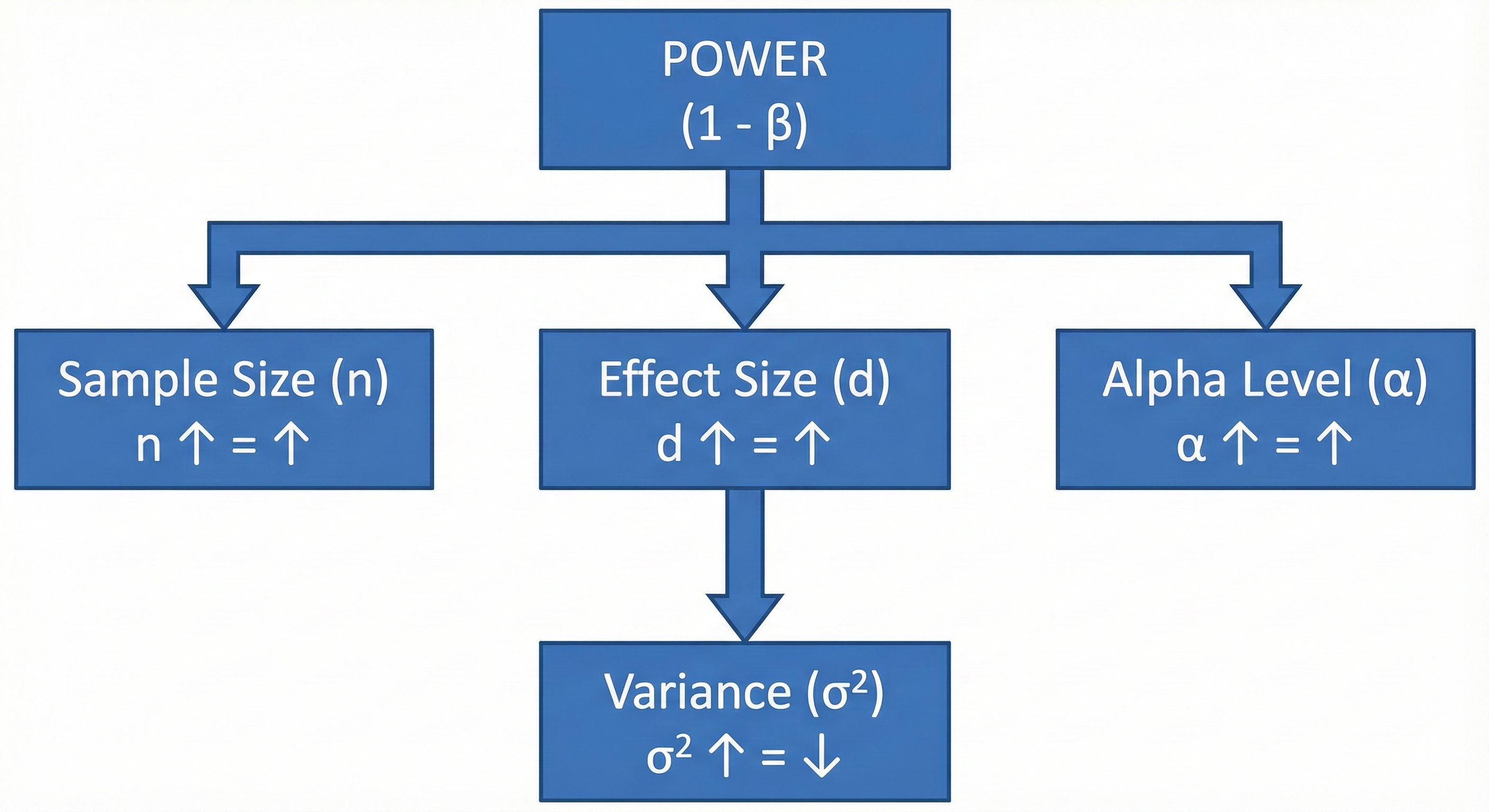
- Sample size (n): Larger samples = More power
- Effect size (d): Larger effects = Easier to detect = More power
- Significance level (α): Higher α = More power (but more false positives)
- Variance (σ²): More variability = Harder to detect signal = Less power
5.3. How Much Power Do You Need?
Convention: Aim for at least 80% power (β = 0.20)
This means: If there truly is an effect, you have an 80% chance of detecting it.
A priori power analysis: Calculate required sample size BEFORE collecting data Post-hoc power analysis: ⚠️ Generally discouraged (see Statistical Sins chapter)
6. 1.5 Degrees of Freedom: The Hidden Constraint
6.1. What Are Degrees of Freedom?
Degrees of freedom (df) = The number of independent values that can vary in your calculation
The Party Seating Analogy:
Imagine you're seating 5 guests at a round table with 5 chairs.
- Guest 1: Can sit anywhere (5 choices)
- Guest 2: Can sit in any of 4 remaining chairs
- Guest 3: 3 remaining chairs
- Guest 4: 2 remaining chairs
- Guest 5: Only 1 chair left — NO CHOICE!
You had freedom for 4 guests; the 5th was constrained. df = 5 - 1 = 4
6.2. Why Degrees of Freedom Matter
Different statistical distributions are actually families of distributions, with df as the parameter that determines the exact shape:
6.3. Common Degrees of Freedom Formulas
| Test | Degrees of Freedom |
|---|---|
| One-sample t-test | n - 1 |
| Independent samples t-test | n₁ + n₂ - 2 |
| Paired samples t-test | n - 1 (n = number of pairs) |
| One-way ANOVA (between groups) | k - 1 (k = number of groups) |
| One-way ANOVA (within groups) | N - k (N = total observations) |
| Chi-square test | (rows - 1) × (columns - 1) |
| Correlation | n - 2 |
Chapter 2: Understanding Distributions — The Shape of Your Data
Before selecting a statistical test, you must understand your data's distribution. This chapter covers the probability distributions you'll encounter most frequently.
7. 2.1 Why Distributions Matter
Every statistical test makes assumptions about how your data is distributed. Use the wrong test for your distribution, and your results may be meaningless.
The Key Question: If I could collect infinite samples, what shape would the histogram take?
8. 2.2 The Normal (Gaussian) Distribution
8.1. The Bell Curve — Queen of Distributions
Why it's special: Thanks to the Central Limit Theorem, the average of many independent random variables tends toward normal distribution, regardless of the original distribution. This is why it appears everywhere.
8.2. Mathematical Formula
Breaking it down:
- μ (mu): Mean — the center of the bell
- σ (sigma): Standard deviation — the "width" of the bell
- e: Euler's number (~2.718)
- π: Pi (~3.14159)
Intuitive understanding: The formula says "the probability density decreases exponentially as you move away from the mean, with the rate of decrease controlled by the standard deviation."
8.3. The 68-95-99.7 Rule (Empirical Rule)
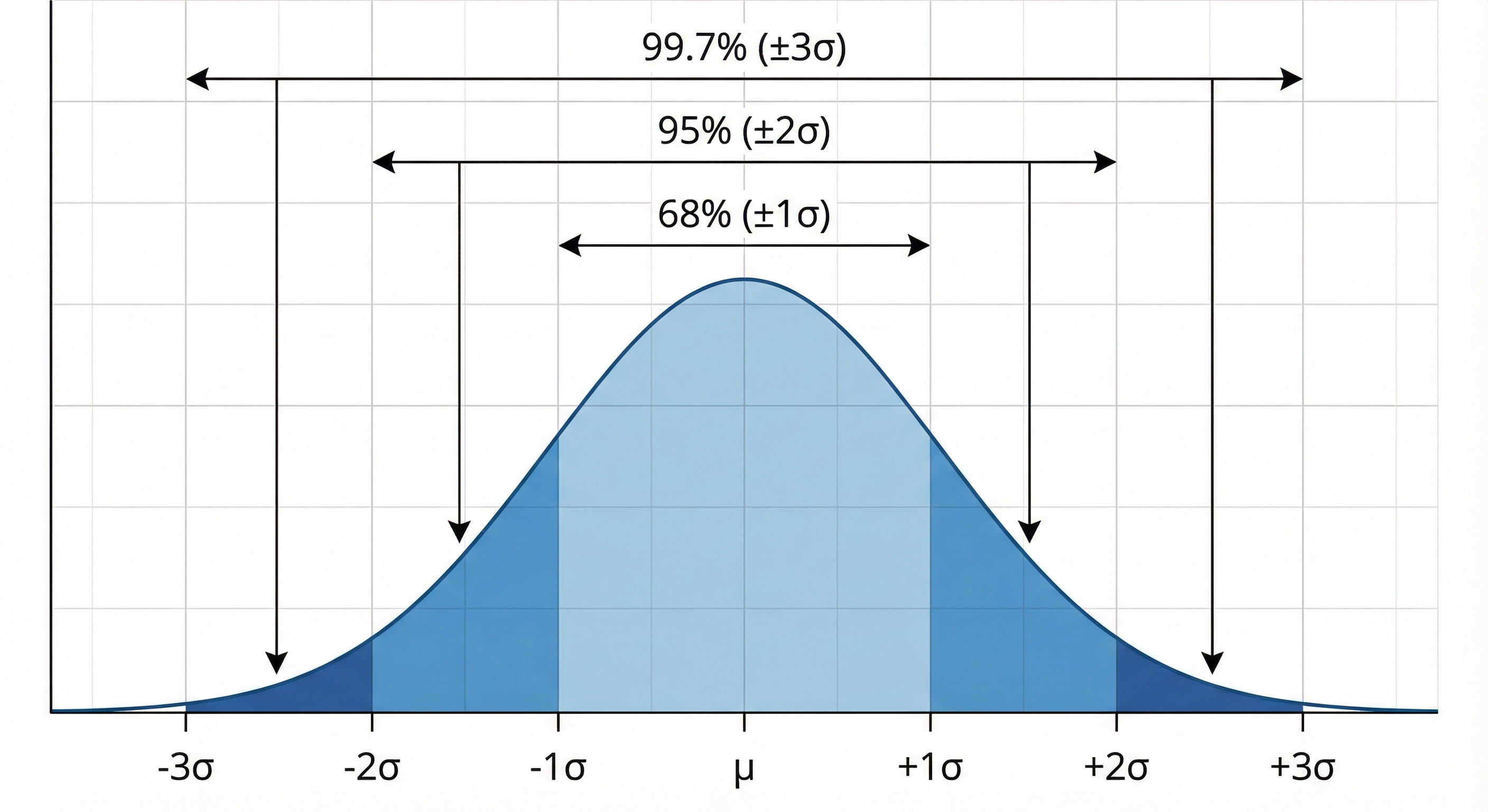
- 68% of data falls within ±1 standard deviation
- 95% of data falls within ±2 standard deviations
- 99.7% of data falls within ±3 standard deviations
8.4. Real-World Examples
- Human height (within a sex)
- IQ scores
- Measurement errors
- Blood pressure readings
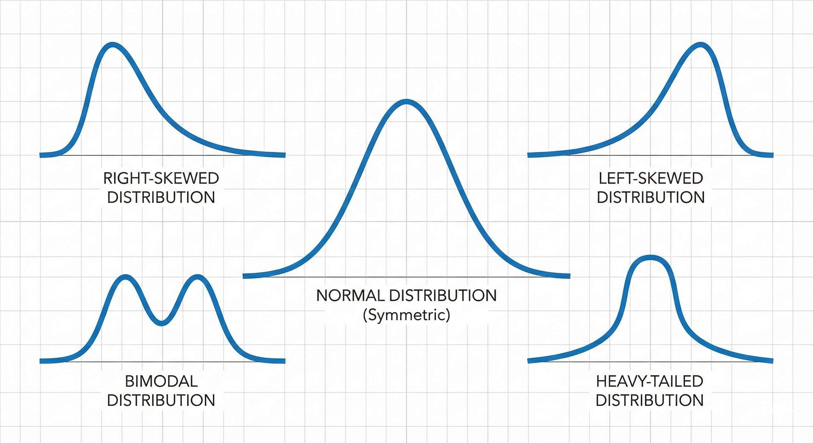
8.5. When Data is NOT Normal
Your data might not be normal if:
- It's bounded (can't go below 0, like reaction times)
- It has heavy tails (extreme values more common)
- It's skewed (asymmetric)
- It's multimodal (multiple peaks)
9. 2.3 The t-Distribution
9.1. The Normal Distribution's Cautious Cousin
When you need it: When you're estimating a population mean but:
- Sample size is small (typically n < 30)
- Population standard deviation is unknown (you're estimating it from data)
9.2. How It Differs From Normal
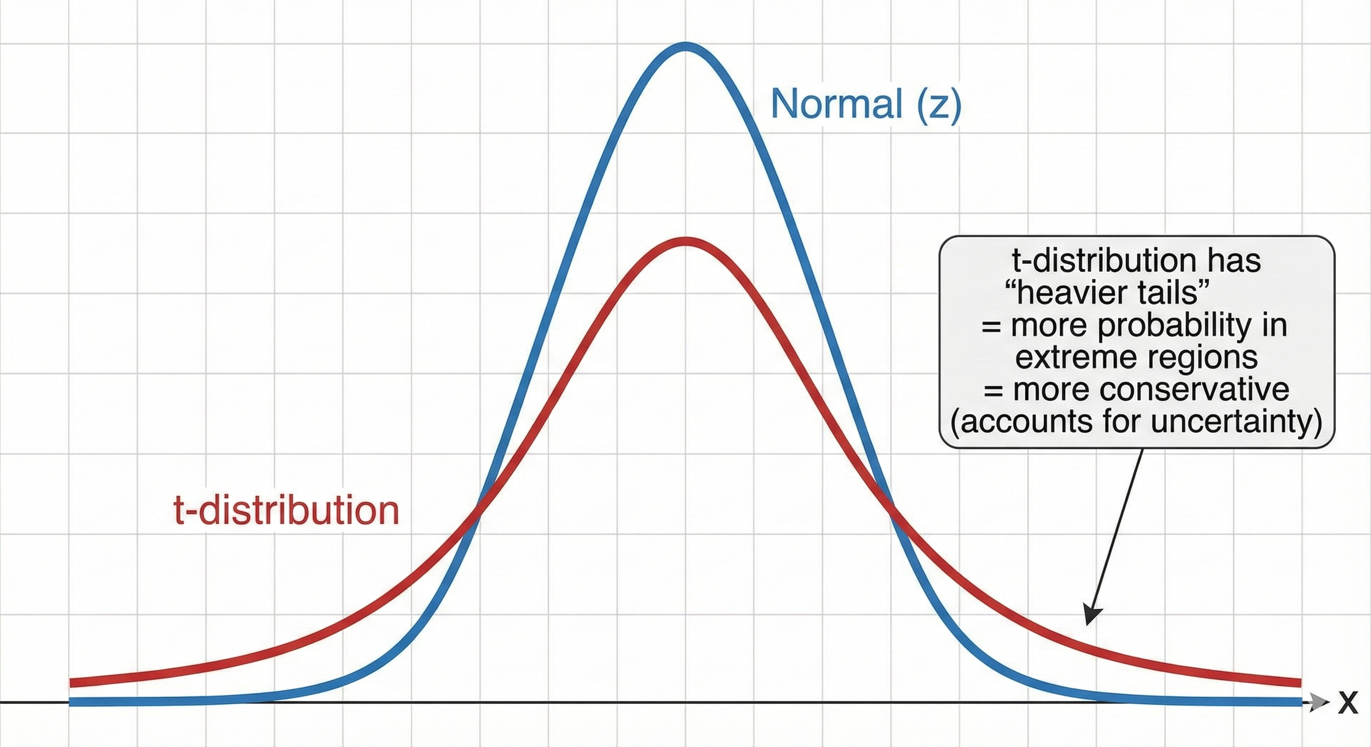
The key insight: With small samples, our estimate of the standard deviation is uncertain. The t-distribution accounts for this extra uncertainty by putting more probability in the tails.
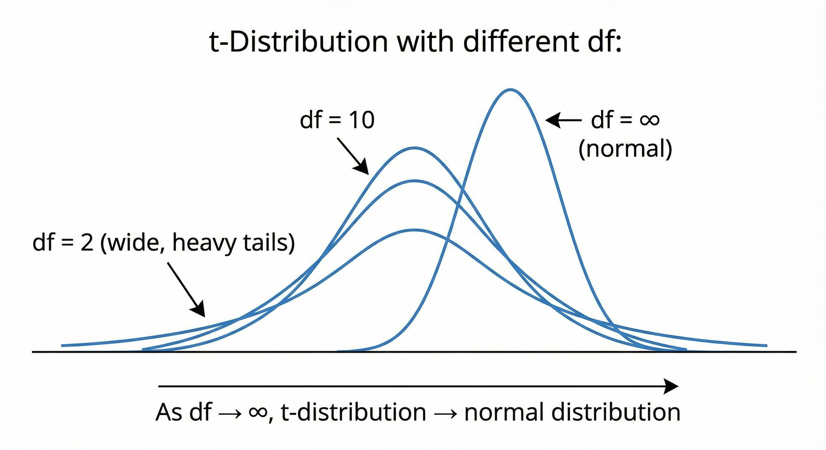
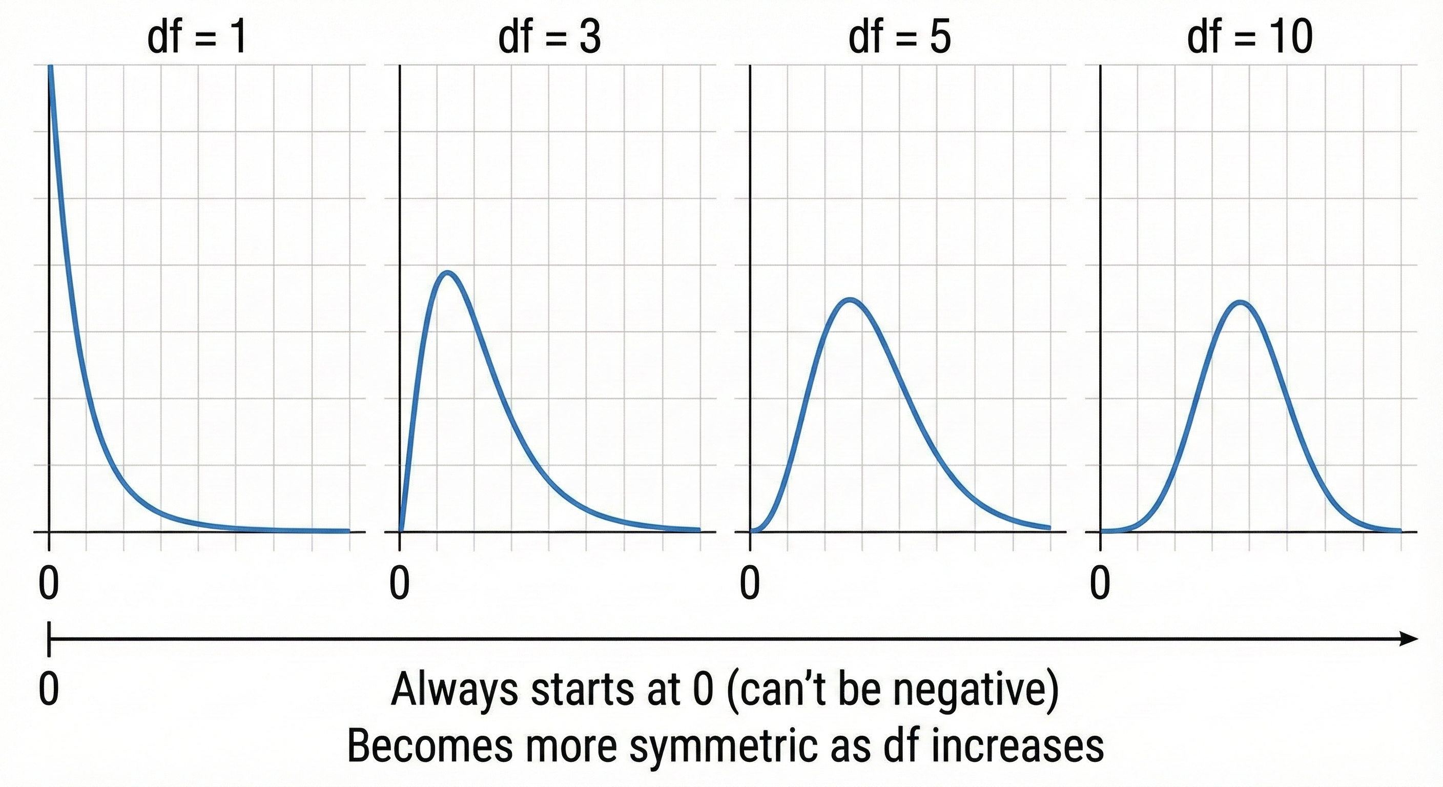
9.3. The Shape Parameter: Degrees of Freedom
As df increases, t-distribution → normal distribution
| df | How close to normal? |
|---|---|
| 1 | Very different (Cauchy distribution) |
| 5 | Noticeably heavier tails |
| 30 | Nearly indistinguishable |
| ∞ | Exactly normal |
10. 2.4 The Chi-Square (χ²) Distribution
10.1. The Distribution of Squared Deviations
What it represents: The sum of squared standard normal random variables.
where each Zᵢ is a standard normal variable (mean=0, sd=1)
10.2. Shape Characteristics
Key properties:
- Always ≥ 0 (it's a sum of squares!)
- Right-skewed, especially for low df
- Mean = df
- Variance = 2 × df
10.3. Where You'll Encounter It
- Chi-square test for independence
- Goodness-of-fit tests
- Variance tests
- As part of F-distribution
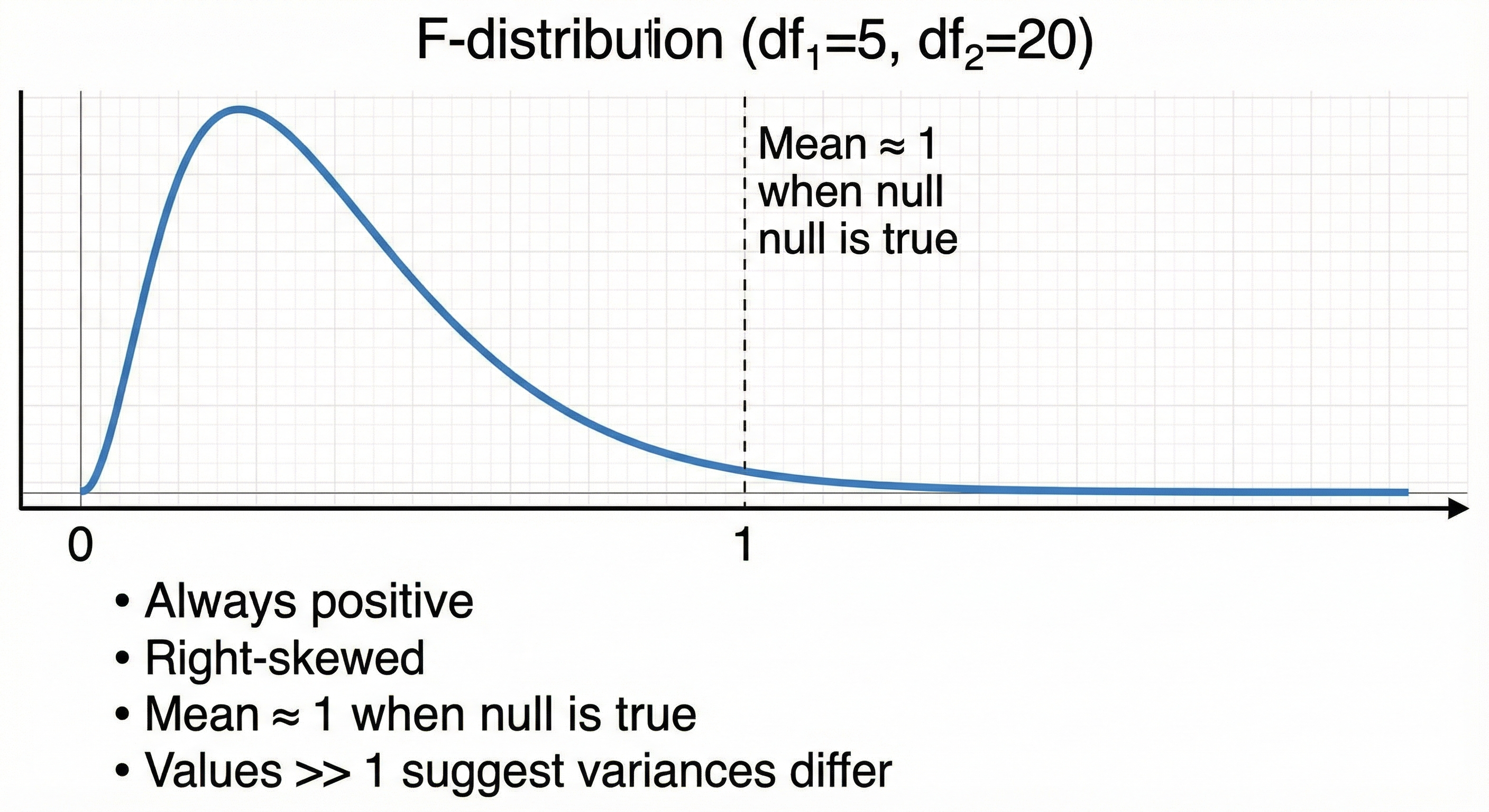
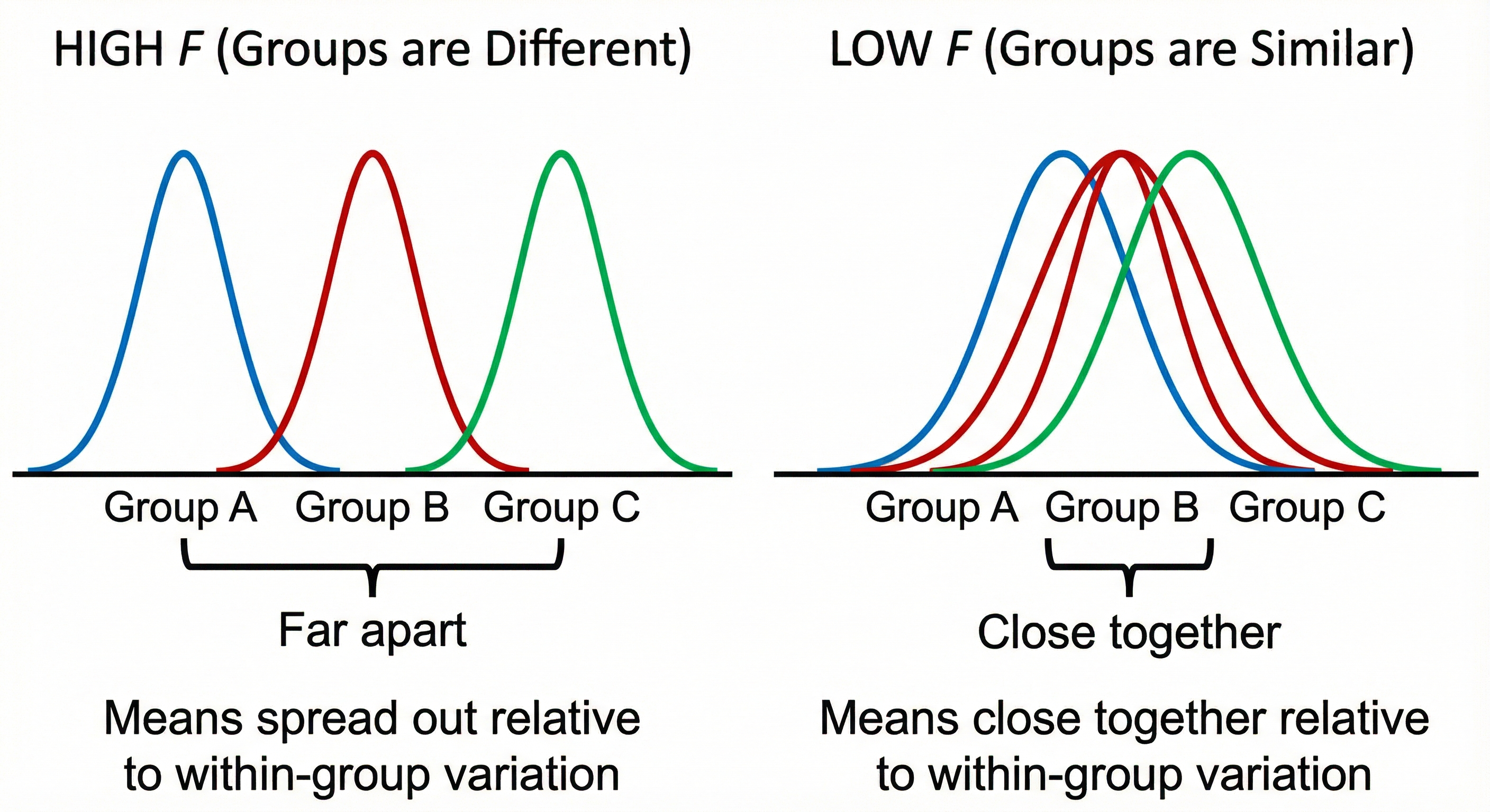
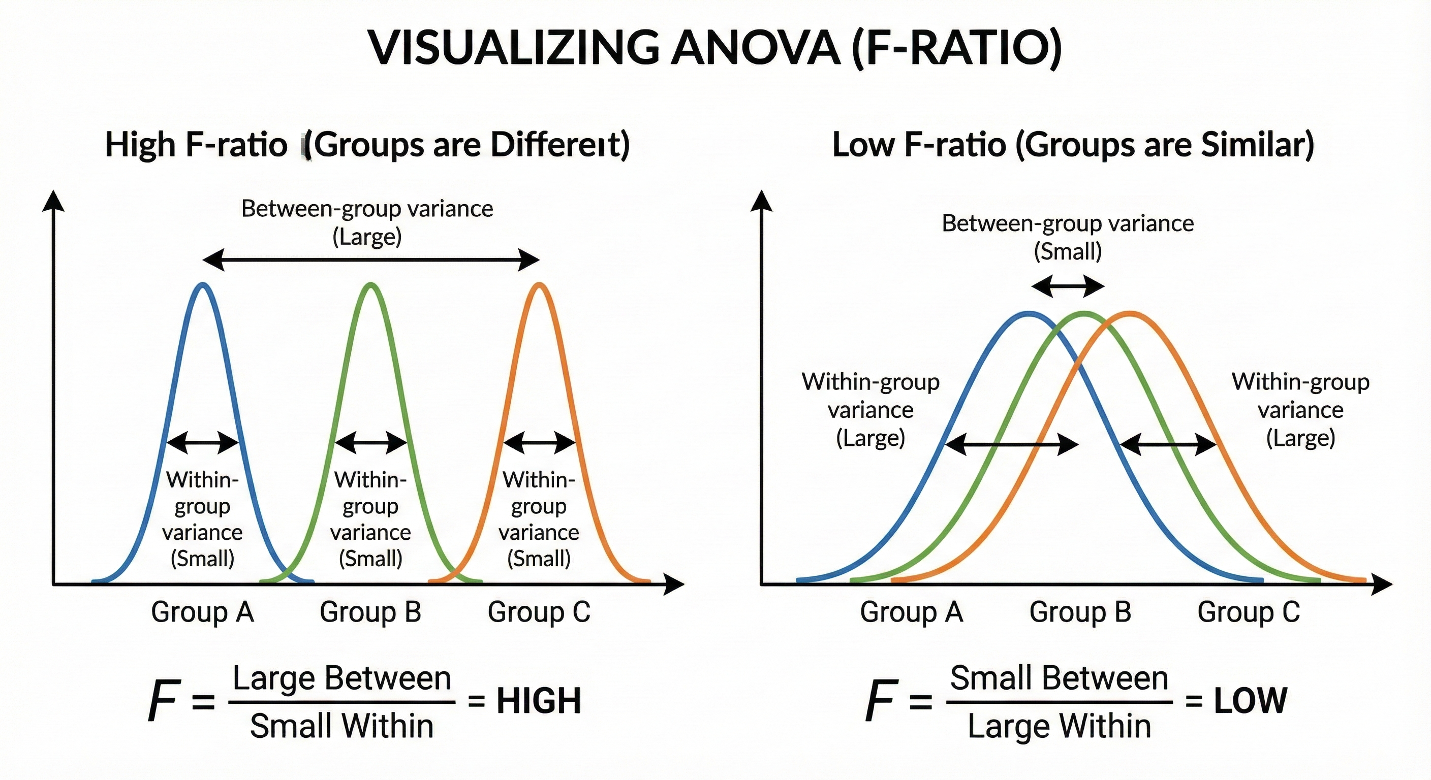
11. 2.5 The F-Distribution
11.1. The Ratio of Two Chi-Squares
What it represents: The ratio of two chi-square distributions (each divided by their df)
Intuition: It compares two variances. How much bigger is one variance relative to another?
11.2. Shape Characteristics
11.3. Where You'll Encounter It
- ANOVA (comparing multiple group means)
- Regression (overall model significance)
- Levene's test (comparing variances)
12. 2.6 Discrete Distributions
12.1. Bernoulli Distribution: Single Yes/No Trial
Parameters: p (probability of success)
Examples: Single coin flip, single survey response (yes/no)
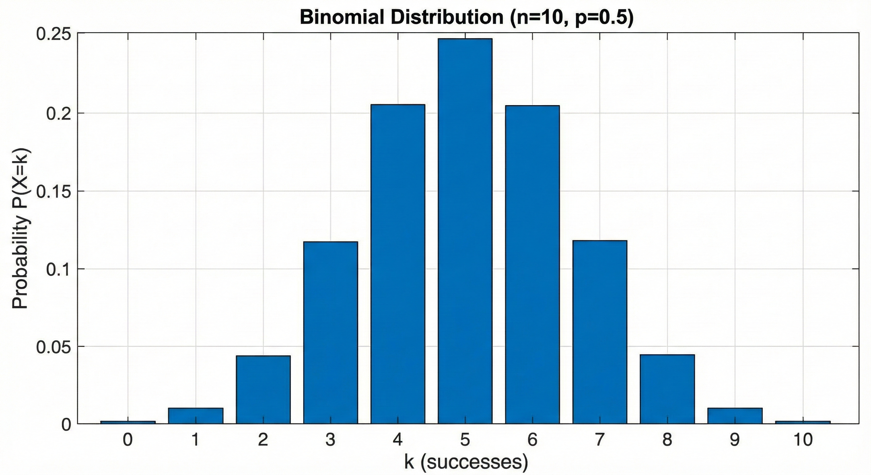
12.2. Binomial Distribution: Multiple Yes/No Trials
Parameters: n (number of trials), p (probability of success per trial)
Formula:
Intuition: "Out of n independent trials, what's the probability of exactly k successes?"
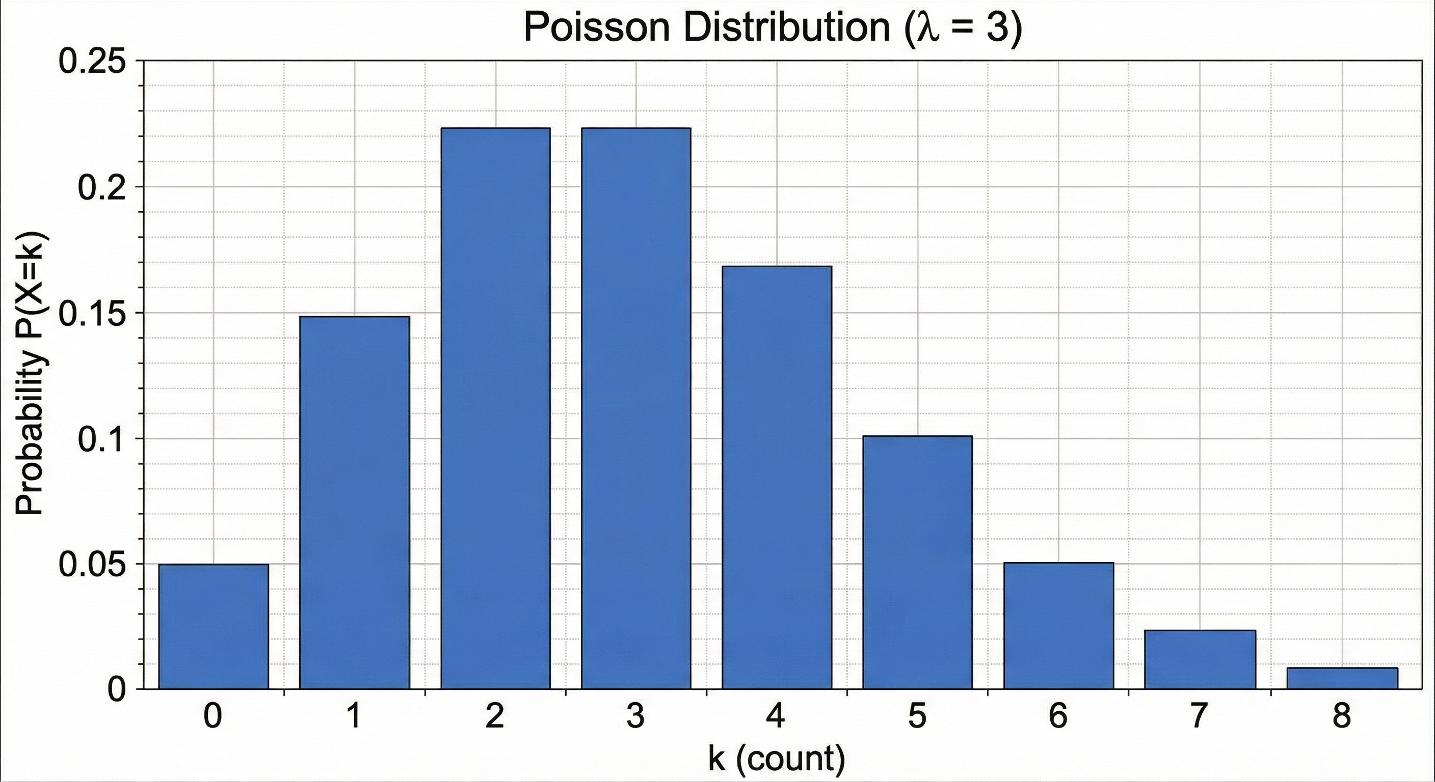
12.3. Poisson Distribution: Counting Rare Events
Parameter: λ (lambda) — average rate of occurrence
Formula:
Use when: Counting events in a fixed interval (time, space, etc.)
- Number of errors per page
- Number of customers per hour
- Number of mutations per genome
13. 2.7 Other Important Distributions
13.1. Exponential Distribution
Use for: Time between events (waiting times)
- Time until next customer arrives
- Time until system failure
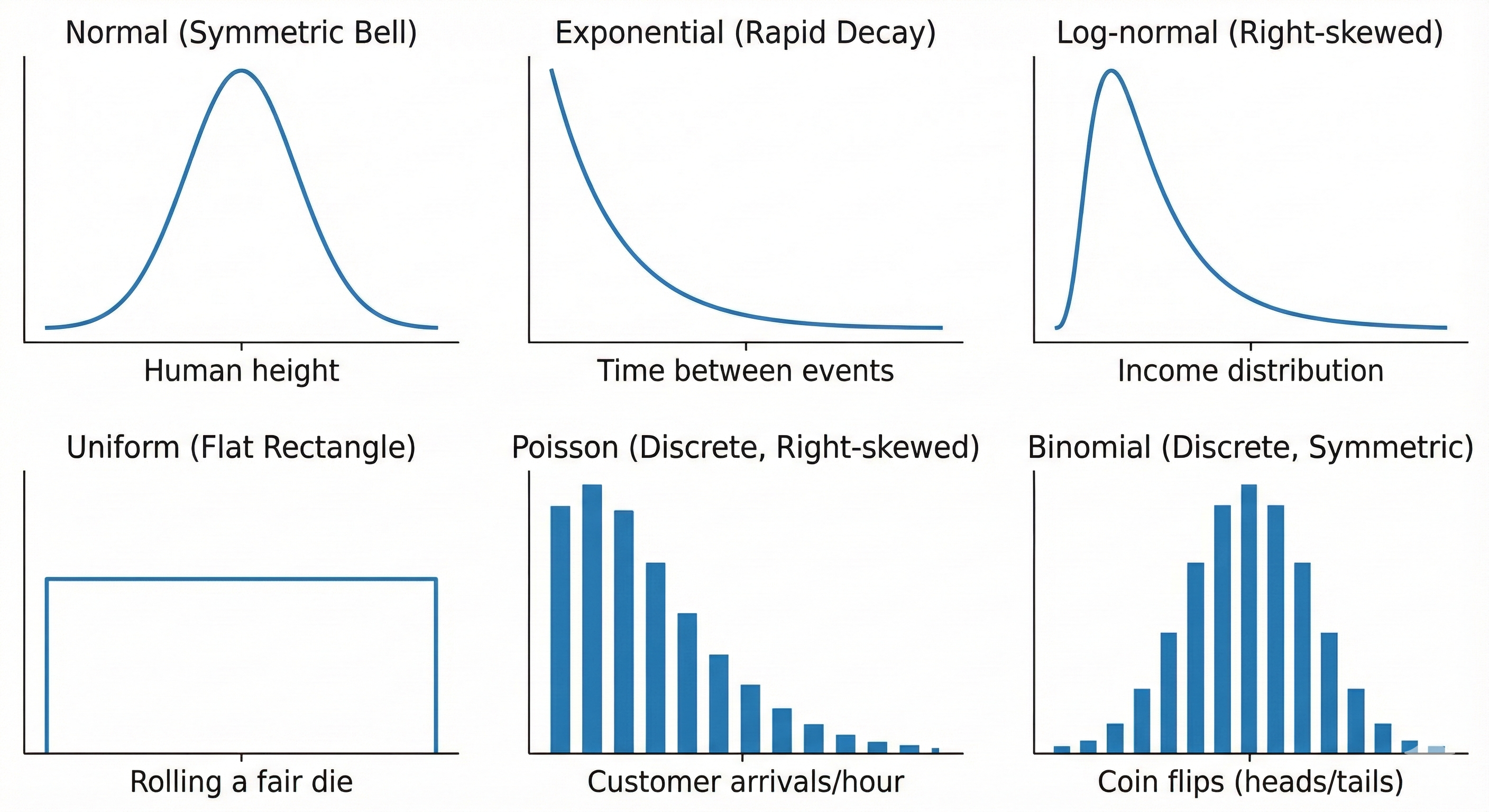
Shape: Starts high at 0, decreases exponentially
13.2. Log-Normal Distribution
Use for: Data that's normal after taking logarithm
- Income distributions
- Reaction times
- Stock prices
Shape: Right-skewed, bounded at 0
13.3. Uniform Distribution
Use for: All values equally likely in a range
- Random number generators
- Rolling a fair die
Shape: Flat rectangle
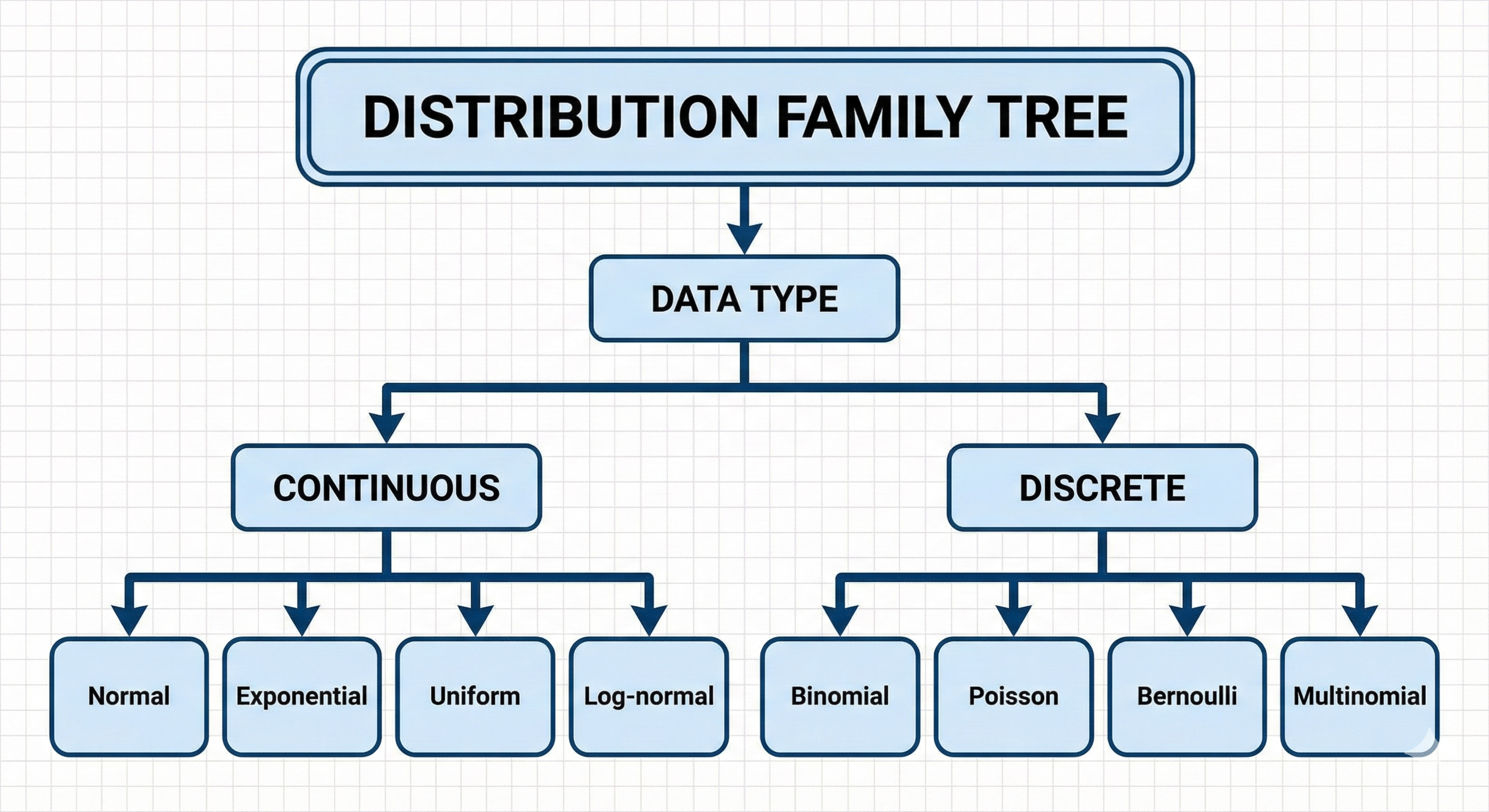
14. 2.8 Distribution Selection Quick Reference
| Your Data Looks Like... | Likely Distribution | Common Tests |
|---|---|---|
| Symmetric bell curve | Normal | t-tests, ANOVA, Pearson |
| Right-skewed, continuous | Log-normal or Exponential | Non-parametric tests, or transform |
| Counts (0, 1, 2, 3...) | Poisson or Binomial | Chi-square, Poisson regression |
| Yes/No outcomes | Bernoulli/Binomial | Chi-square, logistic regression |
| Rankings | — | Non-parametric tests |
| Bounded scores | Beta | Transform or non-parametric |
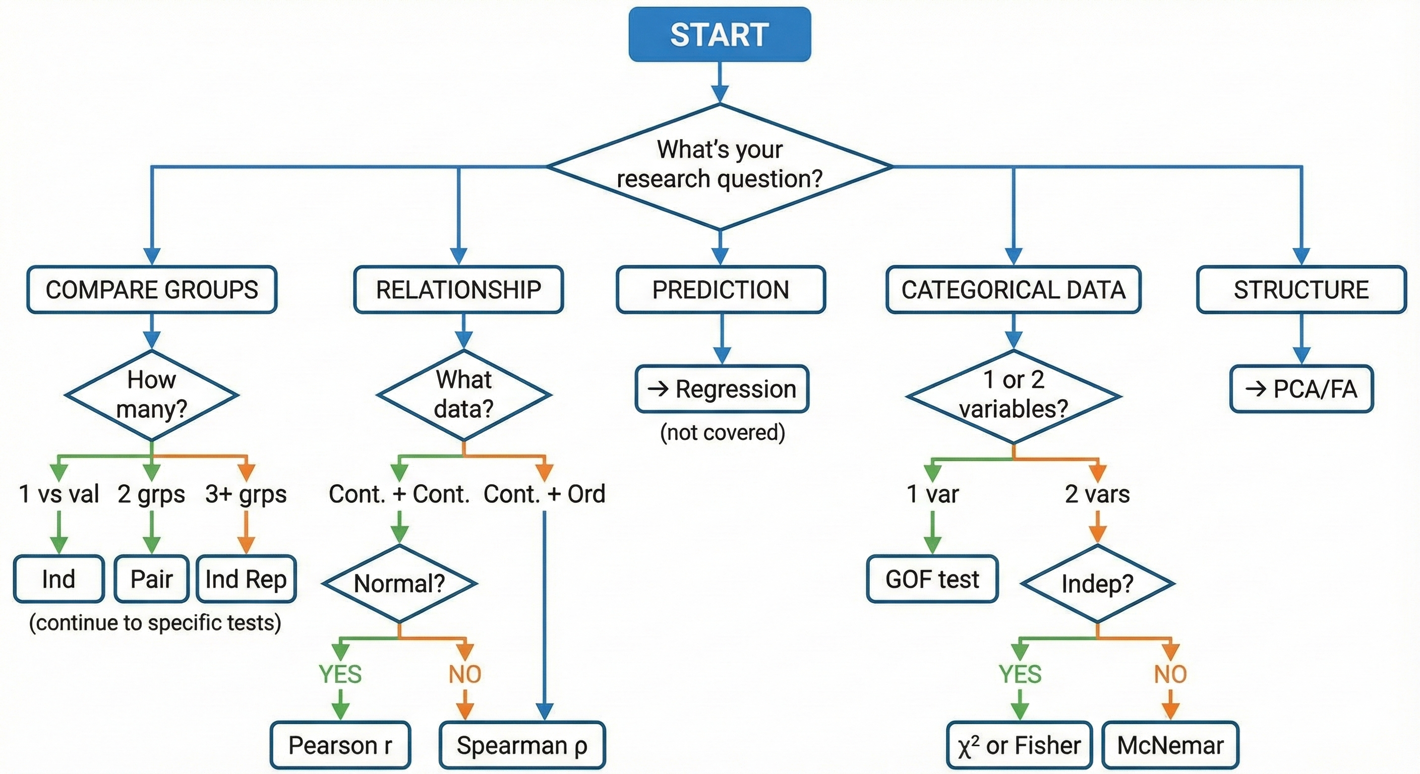
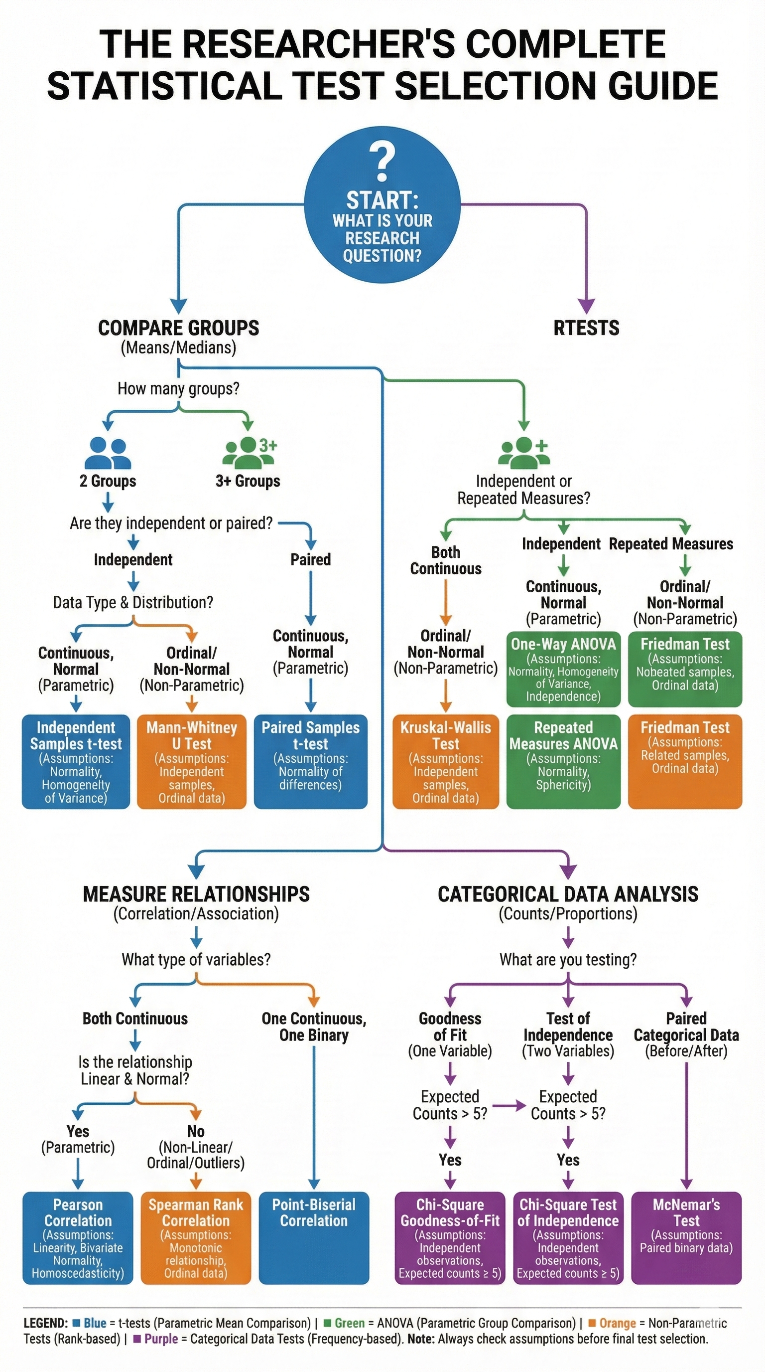
Chapter 3: The Master Decision Tree — Your Navigation System
This is the heart of the guide. Use these decision trees to navigate from "What do I want to know?" to "Which test should I use?"
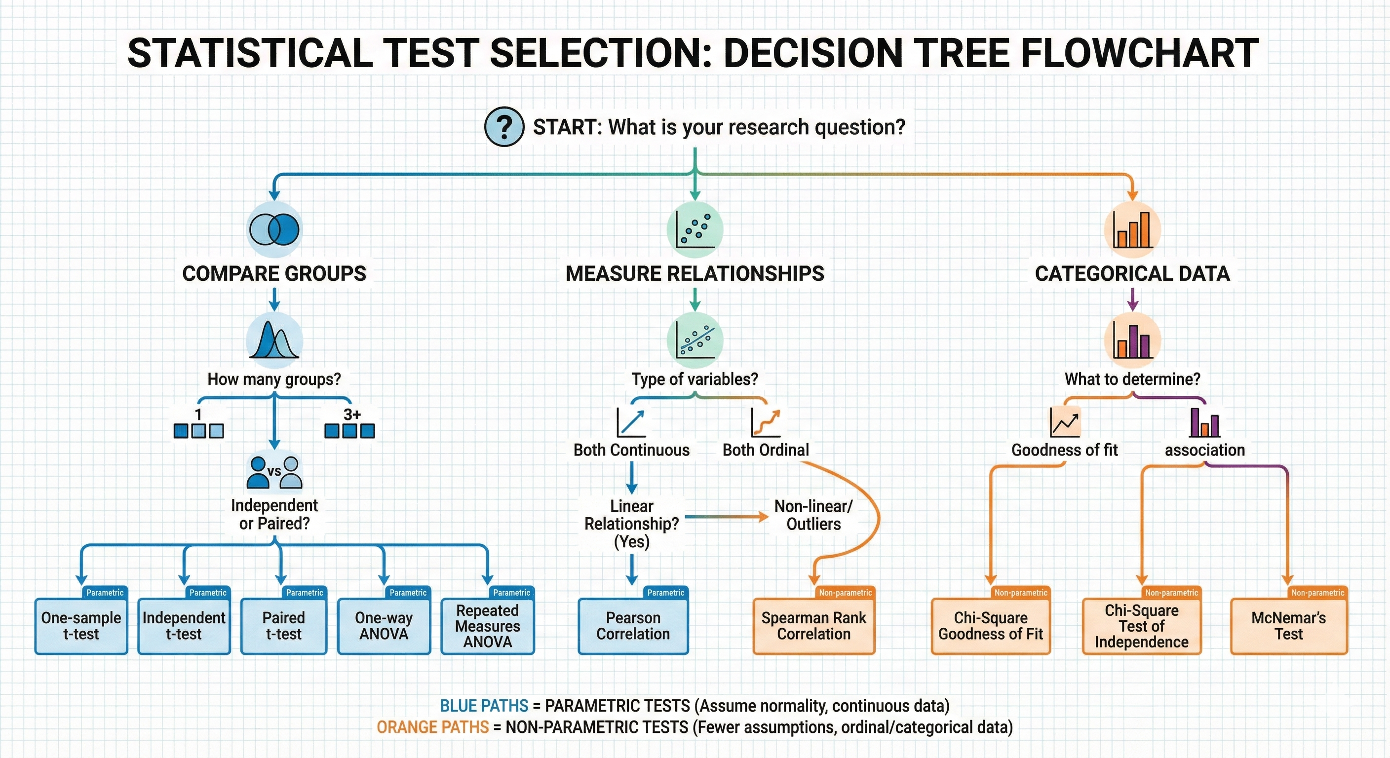
15. 3.1 The Ultimate Decision Tree (ASCII Version)
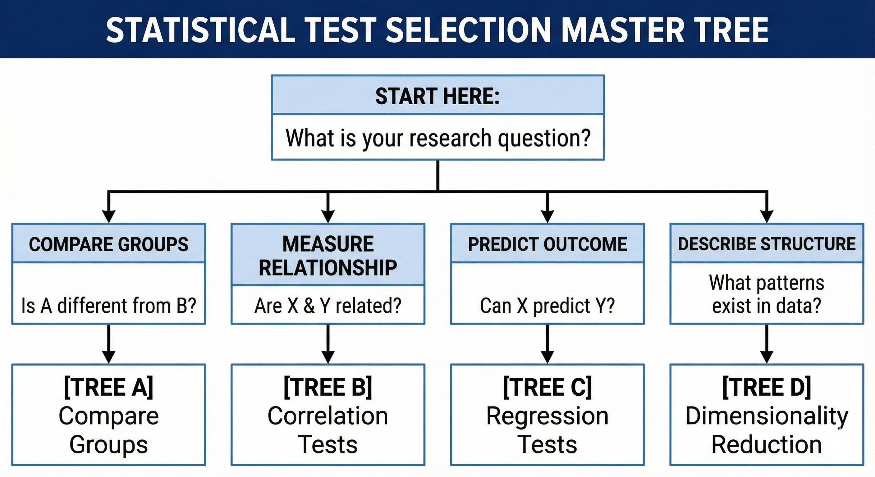
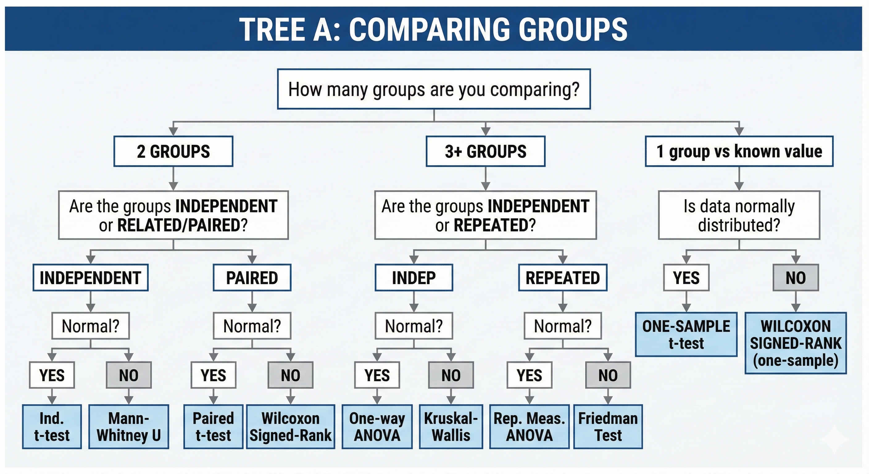
16. 3.2 TREE A: Comparing Groups
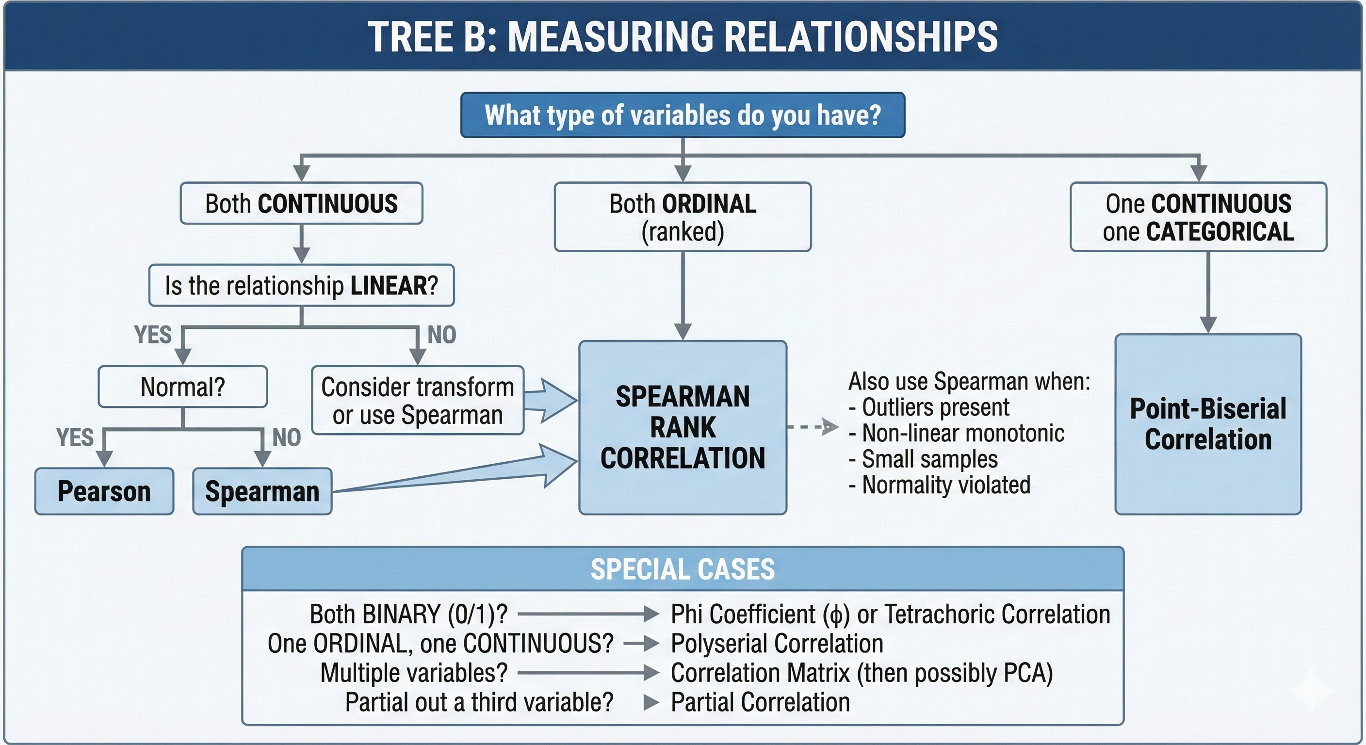
17. 3.3 TREE B: Measuring Relationships (Correlation)
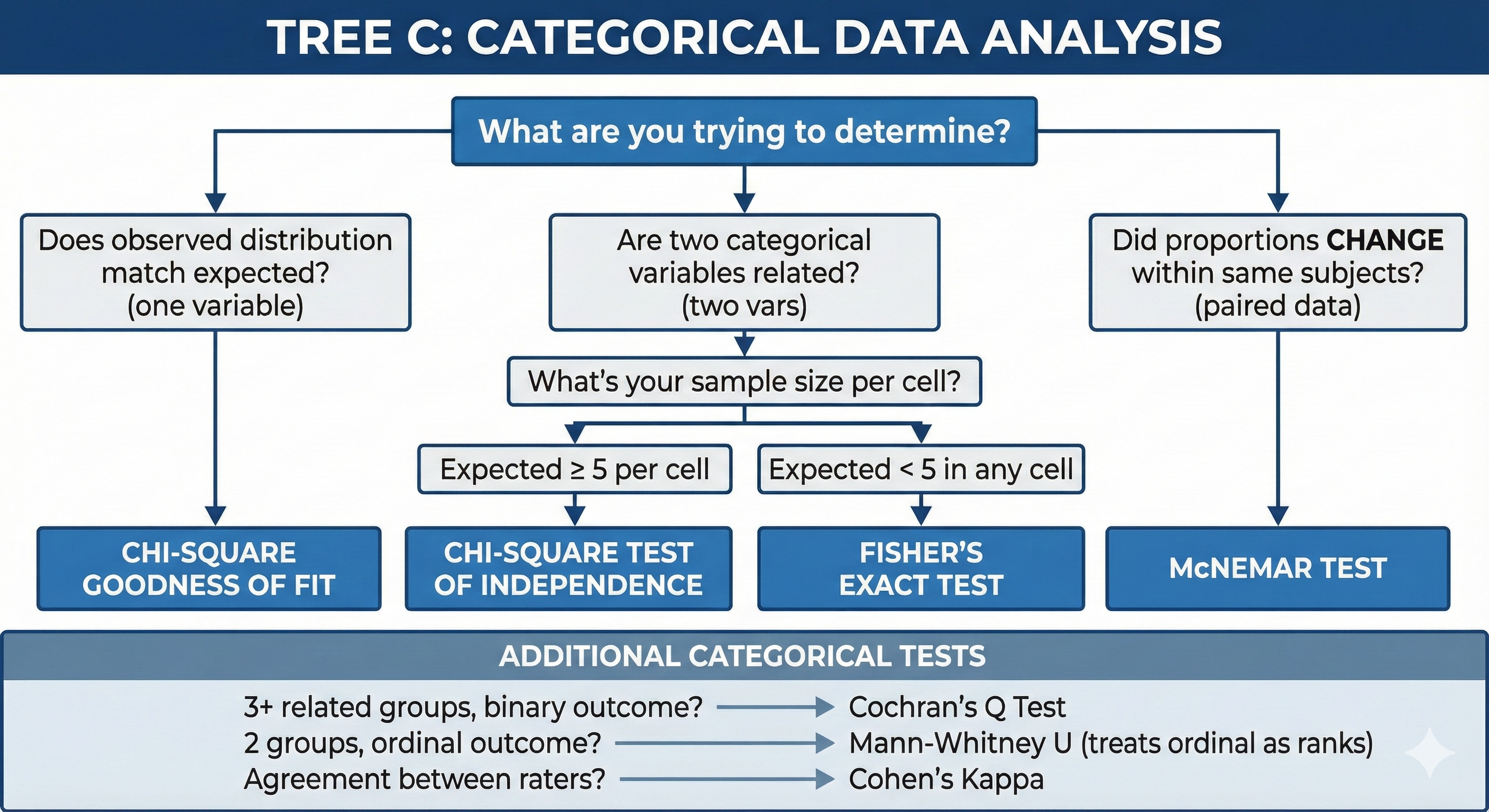
18. 3.4 TREE C: Categorical Data Analysis
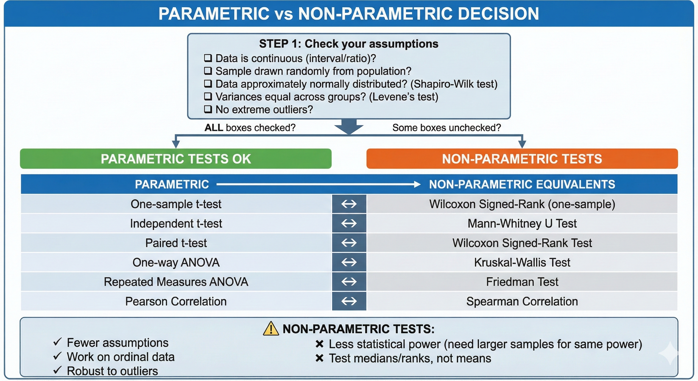
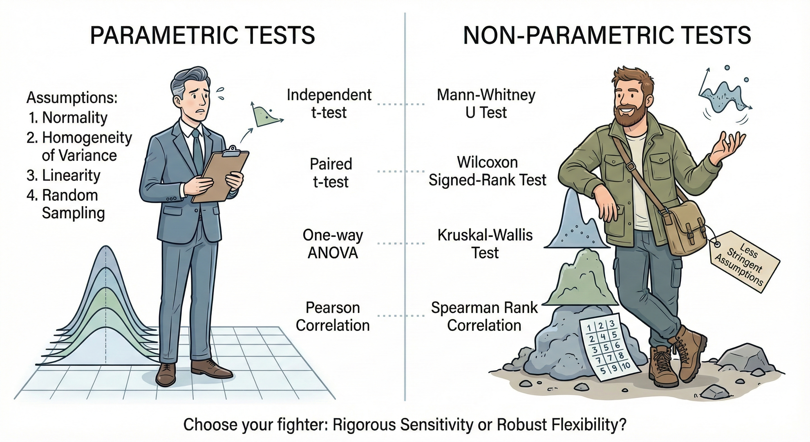
19. 3.5 TREE D: Parametric vs Non-Parametric Decision
Chapter 4: Assumption Testing — The Gates You Must Pass
Before running parametric tests, you must verify their assumptions are met. Think of these tests as gatekeepers that determine which path you can take.
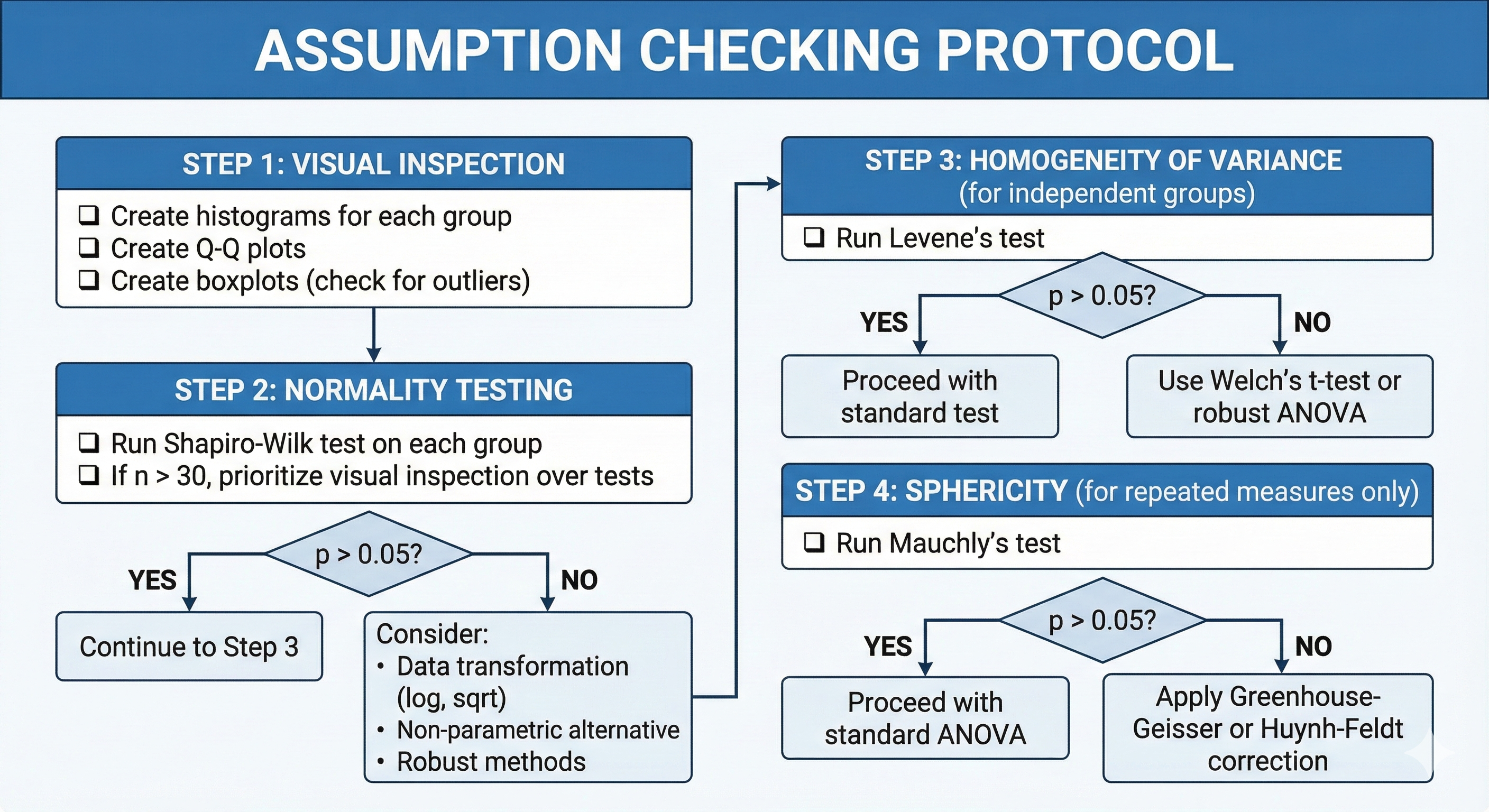
20. 4.1 Testing for Normality
20.1. Shapiro-Wilk Test
Purpose: Tests whether a sample comes from a normally distributed population.
Hypotheses:
- H₀: Data is normally distributed
- H₁: Data is NOT normally distributed
When to use:
- Sample size < 50 (most powerful for small samples)
- ⚠️ With large samples (n > 300), may detect trivial deviations
Interpretation:
- p > 0.05 → Fail to reject H₀ → Data is approximately normal ✓
- p < 0.05 → Reject H₀ → Data is NOT normal ✗
The Formula (conceptual):
Where:
- x₍ᵢ₎ = ordered sample values
- aᵢ = constants generated from means and covariances of order statistics
- W ranges from 0 to 1; values close to 1 suggest normality
⚠️ Don't use this when:
- Sample size > 5000 (use visual inspection instead)
- You have clear theoretical reasons to expect non-normality
20.2. Other Normality Tests
| Test | Best For | Notes |
|---|---|---|
| Shapiro-Wilk | Small samples (n < 50) | Most powerful |
| Kolmogorov-Smirnov | Larger samples | Less powerful than Shapiro-Wilk |
| Anderson-Darling | Medium samples | More sensitive to tails |
| D'Agostino-Pearson | Large samples (n > 20) | Tests skewness and kurtosis separately |
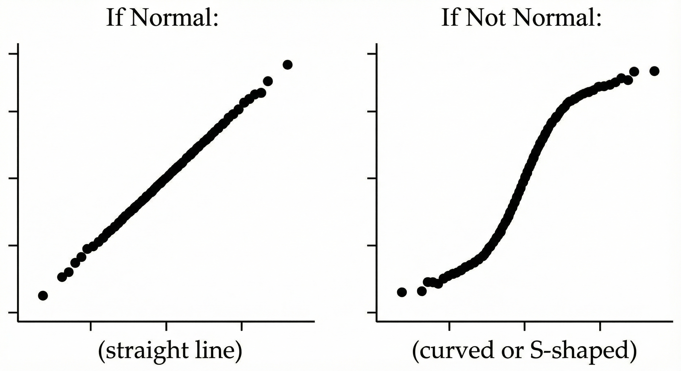
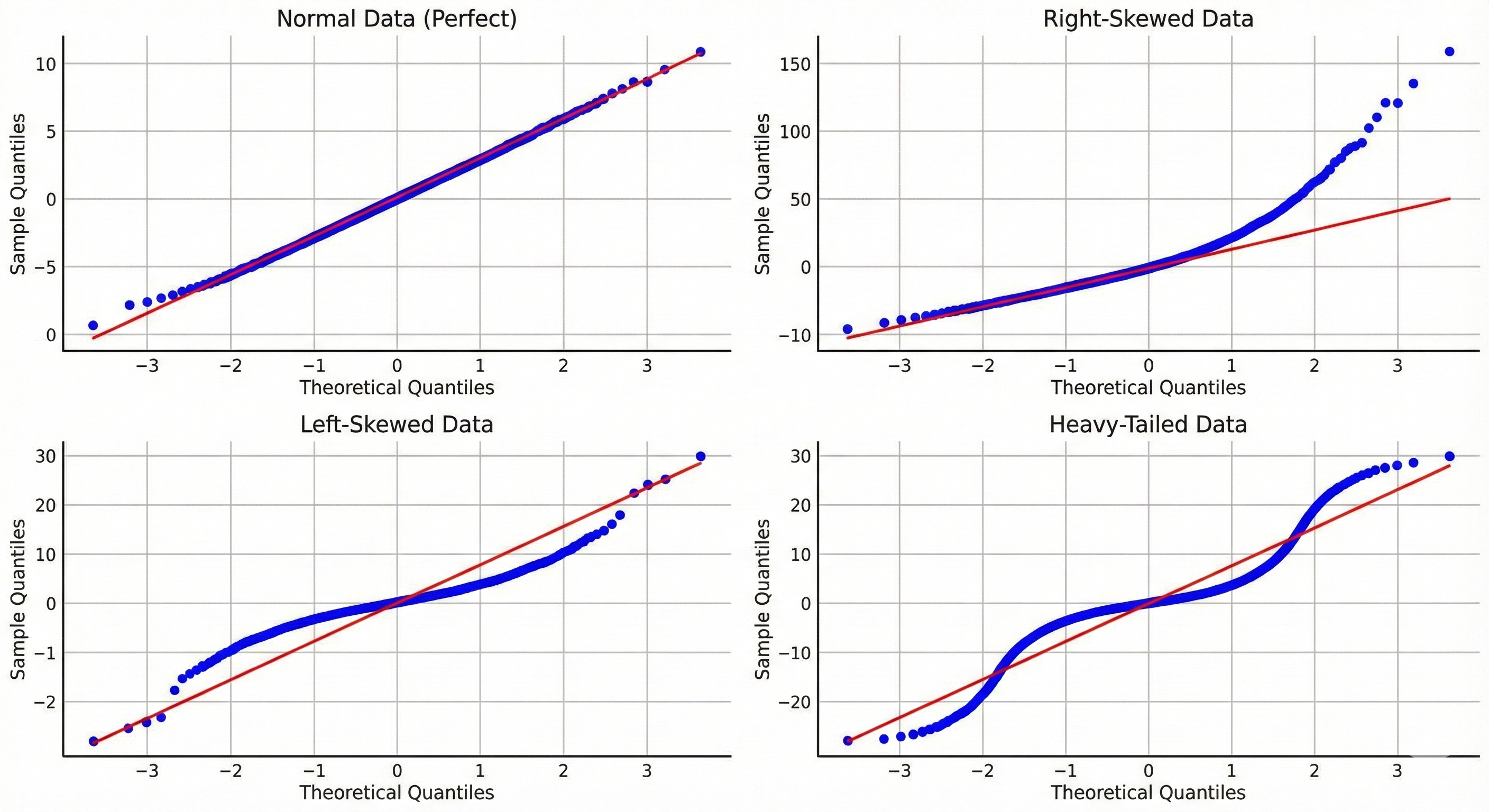
20.3. Visual Methods (Often Better Than Tests!)
Q-Q Plot (Quantile-Quantile Plot):
Histogram with Normal Curve Overlay:
- Visual check for bell shape
- Quick identification of skewness, multiple modes
21. 4.2 Testing for Homogeneity of Variance
21.1. Levene's Test
Purpose: Tests whether variances are equal across groups.
Hypotheses:
- H₀: Variances are equal (homogeneity)
- H₁: Variances are NOT equal (heterogeneity)
When to use:
- Before independent samples t-test or ANOVA
- More robust than Bartlett's test when normality is violated
The Formula:
Where:
- Zᵢⱼ = |Yᵢⱼ - Ȳᵢ| (absolute deviation from group mean)
- k = number of groups
- N = total sample size
Interpretation:
- p > 0.05 → Variances are equal ✓ → Proceed with standard tests
- p < 0.05 → Variances are NOT equal ✗ → Use Welch's t-test or robust ANOVA
21.2. Comparison of Variance Tests
| Test | Assumes Normality? | Robustness |
|---|---|---|
| Levene's (median-based) | No | Most robust |
| Brown-Forsythe | No | Very robust (uses median) |
| Bartlett's | Yes | Sensitive to non-normality |
⚠️ Don't use this when:
- Groups are very unequal in size (ratio > 4:1)
- Running paired/repeated measures designs
22. 4.3 Testing for Sphericity (Repeated Measures)
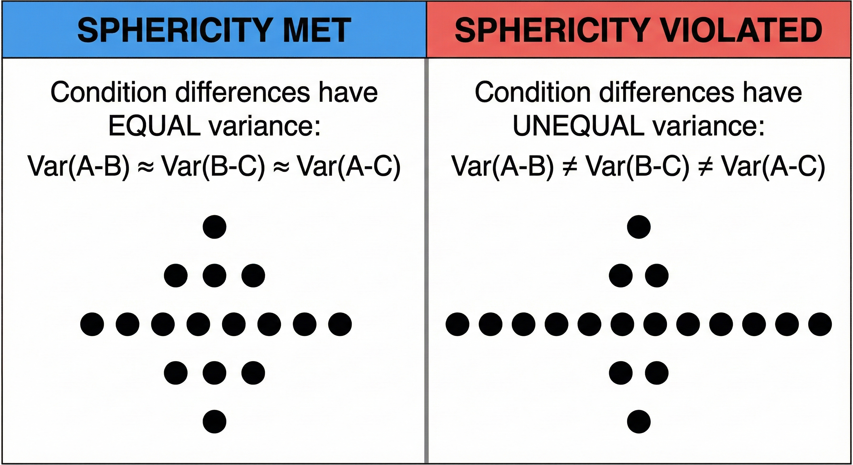
22.1. Mauchly's Test of Sphericity
Purpose: Tests whether the variances of differences between all pairs of conditions are equal. Required assumption for repeated measures ANOVA.
Hypotheses:
- H₀: Sphericity assumption is met
- H₁: Sphericity assumption is violated
When to use:
- Before repeated measures ANOVA
- When you have 3+ repeated conditions
Why sphericity matters:
Interpretation:
- p > 0.05 → Sphericity is met ✓ → Use standard repeated measures ANOVA
- p < 0.05 → Sphericity is violated ✗ → Apply correction:
- Greenhouse-Geisser: Conservative, use when ε < 0.75
- Huynh-Feldt: Less conservative, use when ε ≥ 0.75
The Epsilon (ε) Correction:
- ε = 1.0 means perfect sphericity
- Lower ε means worse violation
- Corrections multiply degrees of freedom by ε, making test more conservative
23. 4.4 Assumption Checking Flowchart
24. 4.5 What To Do When Assumptions Are Violated
24.1. Decision Matrix
| Violation | Minor | Moderate | Severe |
|---|---|---|---|
| Non-normality | Proceed (t-test is robust) | Transform data | Use non-parametric |
| Unequal variances | Use Welch's correction | Use Welch's + bootstrap | Use non-parametric |
| Sphericity | Use Huynh-Feldt | Use Greenhouse-Geisser | Use MANOVA or mixed models |
| Outliers | Winsorize | Trim | Remove and report sensitivity analysis |
24.2. Data Transformations
| Original Distribution | Transformation | When to Use |
|---|---|---|
| Right-skewed | Log(x) | Positive data, multiplicative effects |
| Right-skewed | √x | Count data |
| Right-skewed | 1/x | Extreme skew |
| Left-skewed | x² | Already positive data |
| Proportions | arcsin(√x) | Proportions bounded 0-1 |
⚠️ Caution with transformations:
- Interpretation changes (log-transformed means are geometric means)
- Must transform back for reporting
- May not fully fix violations
Chapter 5: Comparing Groups — The Core Tests
This chapter covers the tests you'll use most frequently: comparing means between groups.
25. Template for Each Test
Every test in this chapter follows this structure:
- What it tests
- When to use it
- Assumptions
- The formula (with intuitive explanation)
- Example
- When NOT to use it
- Reporting format
26. 5.1 The Z-Test
26.1. What It Tests
Tests whether a sample mean differs from a known population mean when the population standard deviation is known.
26.2. When to Use It
- You know the population standard deviation (σ) — rare in practice!
- Large sample size (n ≥ 30)
- Comparing sample to a known benchmark
26.3. Assumptions
- ✓ Population standard deviation is known
- ✓ Data is continuous
- ✓ Random sampling
- ✓ Normal distribution (or large sample)
26.4. The Formula
Breaking it down:
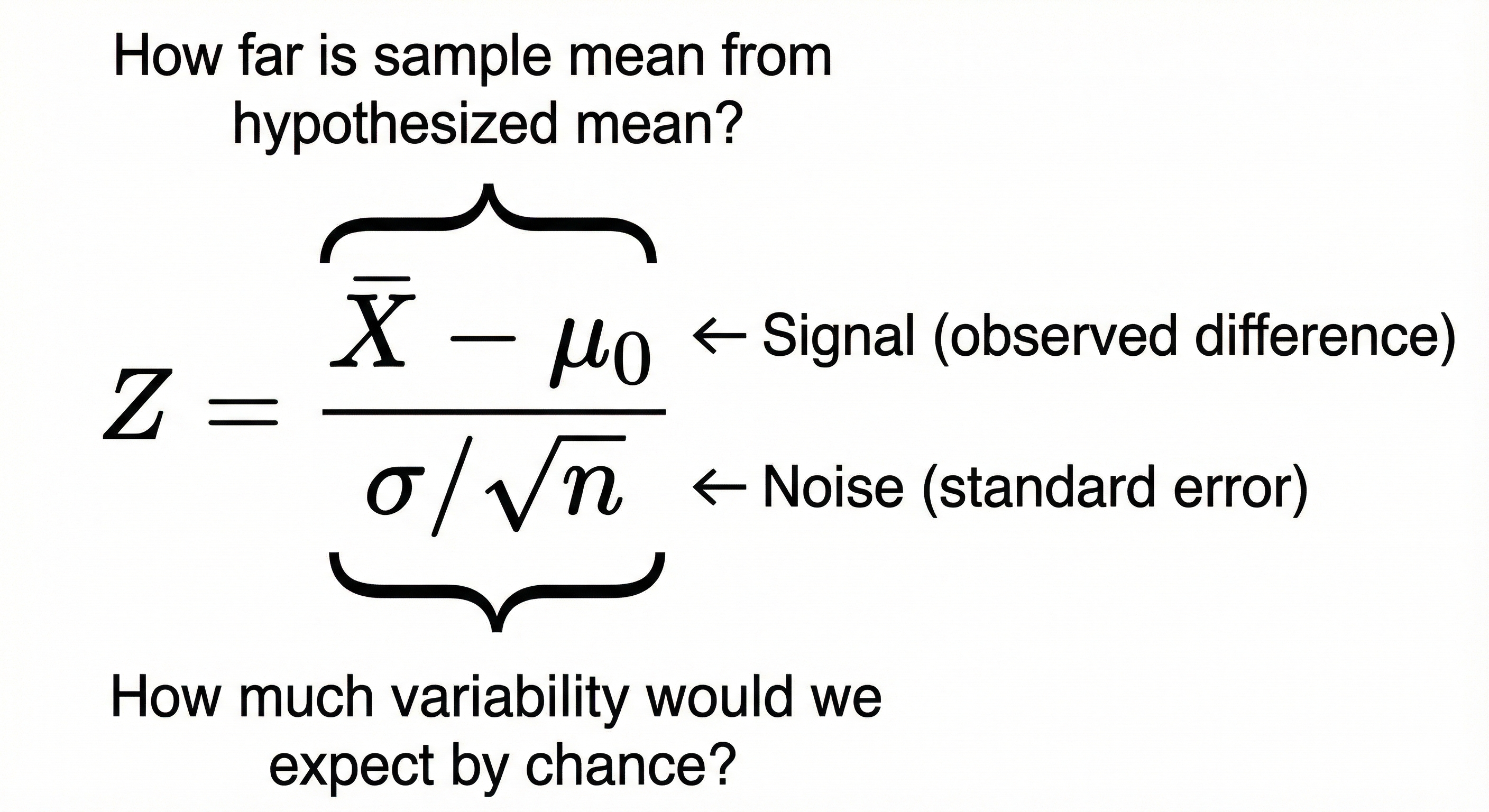
- Numerator: How different is your sample mean from the expected value?
- Denominator: How much random variation would you expect in sample means of this size?
- Z: How many standard errors away from expected is your result?
26.5. Example
Research question: Do users of our new interface complete tasks faster than the industry standard of 120 seconds?
- Sample: n = 36 users
- Sample mean: X̄ = 115 seconds
- Population SD (known from industry data): σ = 18 seconds
Interpretation: The sample mean is 1.67 standard errors below the population mean. Looking up Z = -1.67 in a standard normal table gives p ≈ 0.095 (two-tailed).
Since p > 0.05, we fail to reject H₀. Not enough evidence that our interface differs from the industry standard.
26.6. ⚠️ Don't Use This When
- Population standard deviation is unknown (use t-test instead)
- Sample size is small AND population SD unknown
- Data is clearly non-normal with small n
26.7. Reporting Format
"A one-sample Z-test indicated that task completion time (M = 115s) did not significantly differ from the industry standard of 120s, Z = -1.67, p = .095."
27. 5.2 One-Sample t-Test
27.1. What It Tests
Tests whether a sample mean differs from a known or hypothesized value when population SD is unknown.
27.2. When to Use It
- Comparing a sample to a known/expected value
- Population SD is unknown (estimated from sample)
- Single group, single measurement
27.3. Assumptions
- ✓ Data is continuous (interval/ratio)
- ✓ Random sampling
- ✓ Approximately normal (or n ≥ 30)
- ✓ No extreme outliers
27.4. The Formula
Where:
- X̄ = sample mean
- μ₀ = hypothesized population mean
- s = sample standard deviation
- n = sample size
The only difference from Z-test: We use sample SD (s) instead of population SD (σ)
27.5. Why Degrees of Freedom Matter
When we estimate SD from the sample, we introduce uncertainty. The t-distribution accounts for this by having heavier tails than the normal distribution. With more data (higher df), we're more certain about our SD estimate, and the t-distribution approaches normal.
27.6. Example
Research question: Does our VR experience increase sense of presence compared to the neutral score of 4.0 on a 7-point scale?
- Sample: n = 25 participants
- Sample mean: X̄ = 5.2
- Sample SD: s = 1.5
df = 25 - 1 = 24
Looking up t = 4.0 with df = 24: p < 0.001
Interpretation: The presence score is significantly above the neutral point.
27.7. ⚠️ Don't Use This When
- Data is clearly non-normal (use Wilcoxon signed-rank)
- You have severe outliers
- Data is ordinal (ranks)
- You're comparing two groups (use two-sample t-test)
27.8. Reporting Format
"A one-sample t-test revealed that presence scores (M = 5.2, SD = 1.5) were significantly above the neutral point of 4.0, t(24) = 4.00, p < .001, d = 0.80."
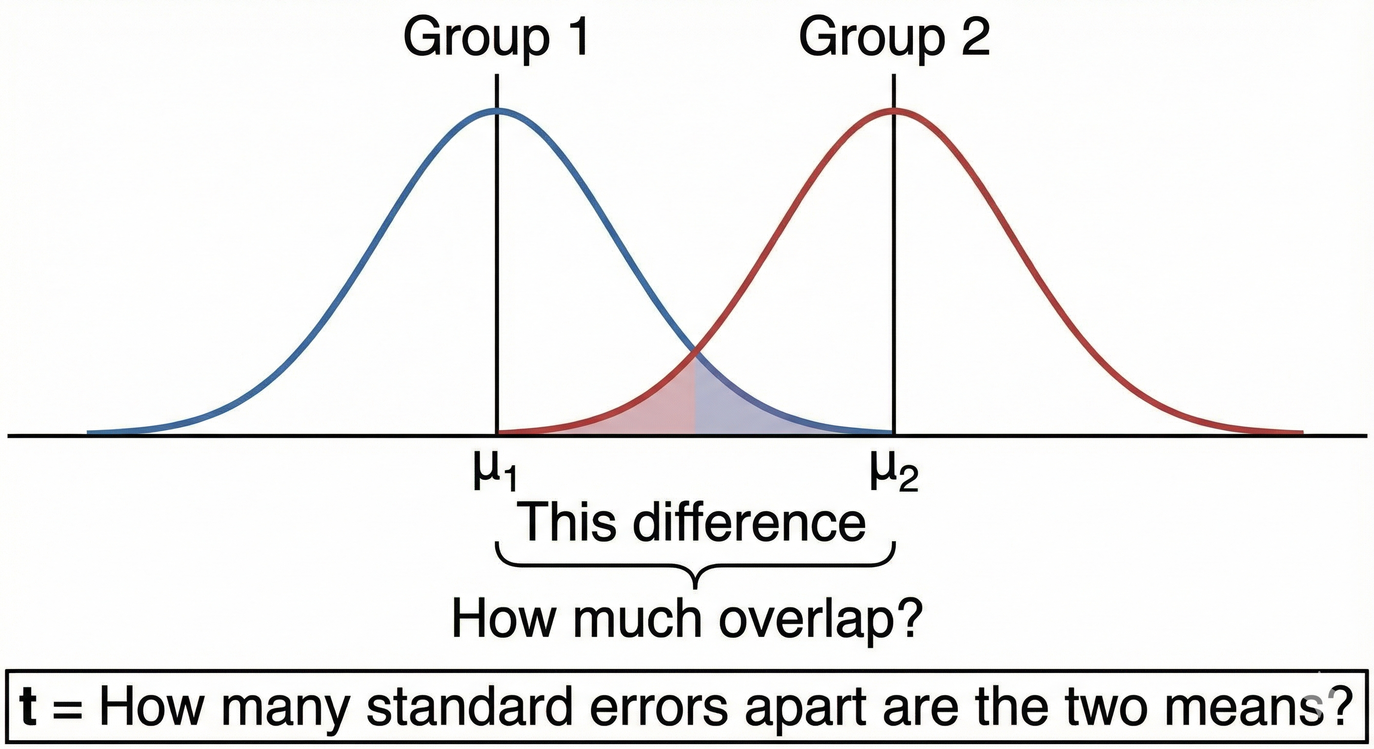
28. 5.3 Independent Samples t-Test
28.1. What It Tests
Tests whether the means of two independent groups differ.
28.2. When to Use It
- Two separate groups (e.g., treatment vs. control)
- Groups are independent (different people)
- Comparing one continuous outcome
28.3. Assumptions
- ✓ Independence between groups
- ✓ Data is continuous
- ✓ Normal distribution in each group (or n ≥ 30 per group)
- ✓ Homogeneity of variance (equal variances)
28.4. The Formula
Standard (equal variances assumed):
Where pooled variance is:
Welch's t-test (unequal variances):
28.5. Geometric Interpretation
28.6. Example
Research question: Do users learn faster with gamified tutorials vs. traditional tutorials?
| Gamified | Traditional | |
|---|---|---|
| n | 20 | 20 |
| Mean (minutes) | 15.3 | 22.1 |
| SD | 4.2 | 5.1 |
Levene's test: p = 0.31 (variances are equal ✓)
Pooled variance:
df = 38, p < .001
Interpretation: Gamified tutorials led to significantly faster learning.
28.7. ⚠️ Don't Use This When
- The same people are in both groups (use paired t-test)
- You have more than 2 groups (use ANOVA)
- Severe violation of normality with small samples (use Mann-Whitney U)
- Variances are very unequal AND unequal n (use Welch's t-test)
28.8. Reporting Format
"An independent samples t-test showed that gamified tutorials (M = 15.3, SD = 4.2) led to significantly faster completion times than traditional tutorials (M = 22.1, SD = 5.1), t(38) = -4.60, p < .001, d = 1.46."
29. 5.4 Paired Samples t-Test
29.1. What It Tests
Tests whether the mean difference between paired observations is zero.
29.2. When to Use It
- Same participants measured twice (pre/post)
- Matched pairs (twins, matched controls)
- Repeated measurements on same items
29.3. Assumptions
- ✓ Pairs are independent of other pairs
- ✓ Differences are continuous
- ✓ Differences are approximately normal
- ✓ No extreme outliers in differences
29.4. The Formula
Where:
- D = differences for each pair (X₁ - X₂)
- D̄ = mean of differences
- sD = standard deviation of differences
- n = number of pairs
Key insight: We're essentially running a one-sample t-test on the differences!
29.5. Why It's More Powerful Than Independent t-Test
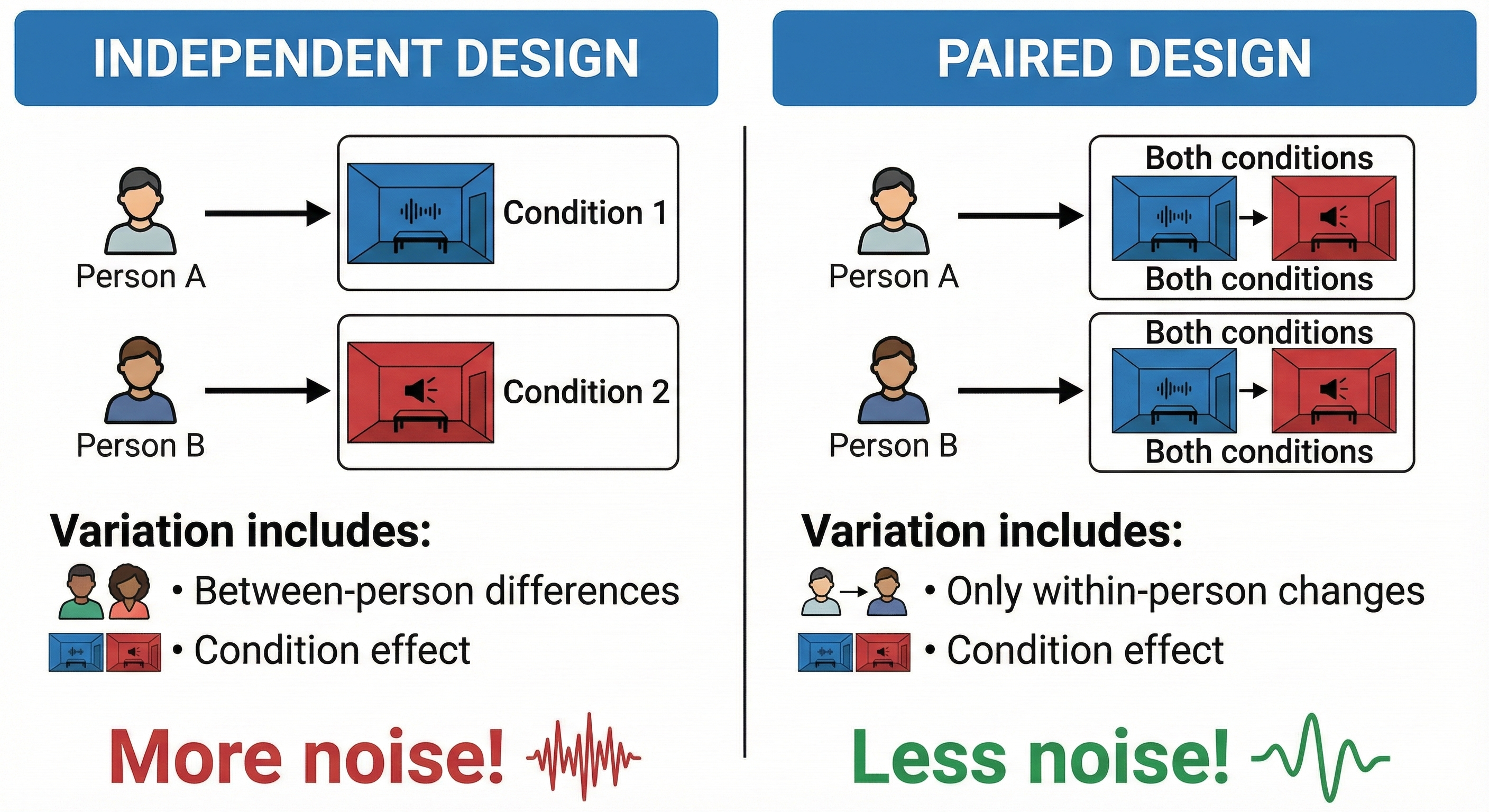
By using each person as their own control, we remove between-person variability.
29.6. Example
Research question: Does a 10-minute mindfulness exercise reduce stress?
| Participant | Before | After | Difference (D) |
|---|---|---|---|
| 1 | 7 | 5 | -2 |
| 2 | 8 | 6 | -2 |
| 3 | 6 | 5 | -1 |
| 4 | 9 | 6 | -3 |
| 5 | 5 | 4 | -1 |
| 6 | 8 | 7 | -1 |
| 7 | 7 | 5 | -2 |
| 8 | 6 | 4 | -2 |
- D̄ = -1.75
- sD = 0.71
- n = 8
df = 7, p < .001
Interpretation: Stress significantly decreased after mindfulness exercise.
29.7. ⚠️ Don't Use This When
- Observations are not truly paired
- Differences are severely non-normal (use Wilcoxon signed-rank)
- You have more than 2 time points (use repeated measures ANOVA)
29.8. Reporting Format
"A paired samples t-test indicated that stress scores significantly decreased from pre-intervention (M = 7.0, SD = 1.3) to post-intervention (M = 5.25, SD = 1.0), t(7) = -6.97, p < .001, d = 1.53."
30. 5.5 Mann-Whitney U Test (Wilcoxon Rank-Sum)
30.1. What It Tests
Tests whether two independent groups come from the same distribution. Non-parametric alternative to independent t-test.
30.2. When to Use It
- Two independent groups
- Data is ordinal OR continuous but non-normal
- Outliers present
- Small samples with uncertain distribution
30.3. Assumptions
- ✓ Independence between groups
- ✓ At least ordinal data
- ✓ Similar shape distributions (if comparing medians)
30.4. The Formula (Conceptual)
- Rank all observations (ignoring group membership)
- Sum the ranks for each group (R₁, R₂)
- Calculate U:
Intuition: U counts how many times a value from one group beats a value from the other group.
30.5. Example
Research question: Do novice users give different usability ratings than experts?
| Novices (Group A) | Experts (Group B) |
|---|---|
| 3 | 7 |
| 4 | 6 |
| 2 | 8 |
| 5 | 9 |
Combined and ranked:
- 2(A)→1, 3(A)→2, 4(A)→3, 5(A)→4, 6(B)→5, 7(B)→6, 8(B)→7, 9(B)→8
R₁ (Novices) = 1+2+3+4 = 10 R₂ (Experts) = 5+6+7+8 = 26
U₁ = 4×4 + 4×5/2 - 10 = 16 + 10 - 10 = 16 U₂ = 4×4 + 4×5/2 - 26 = 16 + 10 - 26 = 0
U = min(U₁, U₂) = 0
Interpretation: With U = 0, there's no overlap at all! Every expert rating exceeded every novice rating. This is highly significant.
30.6. ⚠️ Don't Use This When
- Data meets t-test assumptions (t-test has more power)
- You need to compare means specifically
- You have paired/repeated data (use Wilcoxon signed-rank)
30.7. Reporting Format
"A Mann-Whitney U test revealed that expert usability ratings (Mdn = 7.5) were significantly higher than novice ratings (Mdn = 3.5), U = 0, p = .029, r = .87."
31. 5.6 Wilcoxon Signed-Rank Test
31.1. What It Tests
Tests whether the median difference between paired observations is zero. Non-parametric alternative to paired t-test.
31.2. When to Use It
- Paired/repeated measures data
- Differences are non-normal
- Ordinal data
- Small sample with uncertain distribution
31.3. Assumptions
- ✓ Pairs are independent
- ✓ At least ordinal data
- ✓ Symmetric distribution of differences (for median interpretation)
31.4. The Formula (Conceptual)
- Calculate differences for each pair
- Rank absolute differences (ignore zeros)
- Assign signs based on direction of difference
- Sum positive ranks (W⁺) and negative ranks (W⁻)
- Test statistic: W = min(W⁺, W⁻)
31.5. Example
Research question: Does a UI redesign improve satisfaction scores?
| User | Before | After | Difference | |Diff| | Rank | Signed Rank | |------|--------|-------|------------|--------|------|-------------| | 1 | 3 | 5 | +2 | 2 | 3.5 | +3.5 | | 2 | 4 | 4 | 0 | — | — | — | | 3 | 2 | 5 | +3 | 3 | 5 | +5 | | 4 | 5 | 4 | -1 | 1 | 1 | -1 | | 5 | 3 | 5 | +2 | 2 | 3.5 | +3.5 | | 6 | 2 | 4 | +2 | 2 | 3.5 | +3.5 |
W⁺ = 3.5 + 5 + 3.5 + 3.5 = 15.5 W⁻ = 1 W = 1
Interpretation: The small W⁻ suggests most differences were positive (improvement).
31.6. ⚠️ Don't Use This When
- Data is normal (paired t-test has more power)
- You have independent groups (use Mann-Whitney U)
- You need to compare means specifically
31.7. Reporting Format
"A Wilcoxon signed-rank test indicated that satisfaction scores significantly increased after the redesign, W = 1, p = .046, r = .72."
32. 5.7 One-Way ANOVA
32.1. What It Tests
Tests whether means differ across three or more independent groups.
32.2. When to Use It
- 3+ independent groups
- One continuous outcome variable
- One categorical independent variable (factor)
32.3. Assumptions
- ✓ Independence of observations
- ✓ Normal distribution within each group
- ✓ Homogeneity of variance
- ✓ No extreme outliers
32.4. The Formula (F-ratio)
Where:
32.5. Geometric Interpretation
32.6. The ANOVA Table
| Source | SS | df | MS | F |
|---|---|---|---|---|
| Between | Σnⱼ(X̄ⱼ-X̄)² | k-1 | SS_B/df_B | MS_B/MS_W |
| Within | ΣΣ(Xᵢⱼ-X̄ⱼ)² | N-k | SS_W/df_W | |
| Total | ΣΣ(Xᵢⱼ-X̄)² | N-1 |
32.7. Example
Research question: Does font type affect reading speed?
| Sans-serif | Serif | Decorative |
|---|---|---|
| 120 | 115 | 95 |
| 125 | 118 | 90 |
| 118 | 112 | 88 |
| 122 | 120 | 92 |
| 119 | 117 | 85 |
Group means: 120.8, 116.4, 90.0 Grand mean: 109.07
SS_between = 5×[(120.8-109.07)² + (116.4-109.07)² + (90-109.07)²] = 2,809.73 SS_within = Σ(deviations within groups)² = 154.0
F = (2809.73/2) / (154.0/12) = 1404.87 / 12.83 = 109.5
df_between = 2, df_within = 12, p < .001
Interpretation: Font type significantly affects reading speed.
32.8. Post-Hoc Tests
ANOVA tells you if groups differ, but not which groups. Post-hoc tests determine specific pairwise differences:
| Test | When to Use |
|---|---|
| Tukey HSD | Equal n, all pairwise comparisons |
| Bonferroni | Conservative, few planned comparisons |
| Scheffé | Most conservative, complex comparisons |
| Games-Howell | Unequal variances |
32.9. ⚠️ Don't Use This When
- Only 2 groups (use t-test)
- Same participants across conditions (use repeated measures ANOVA)
- Non-normal data with small n (use Kruskal-Wallis)
- Unequal variances with unequal n (use Welch's ANOVA)
32.10. Reporting Format
"A one-way ANOVA revealed a significant effect of font type on reading speed, F(2, 12) = 109.5, p < .001, η² = .95. Post-hoc Tukey tests showed decorative fonts (M = 90.0) were significantly slower than both sans-serif (M = 120.8, p < .001) and serif (M = 116.4, p < .001)."
33. 5.8 Two-Way ANOVA
33.1. What It Tests
Tests the effects of two independent variables (and their interaction) on a continuous outcome.
33.2. When to Use It
- Two categorical independent variables (factors)
- One continuous dependent variable
- Interested in interaction effects
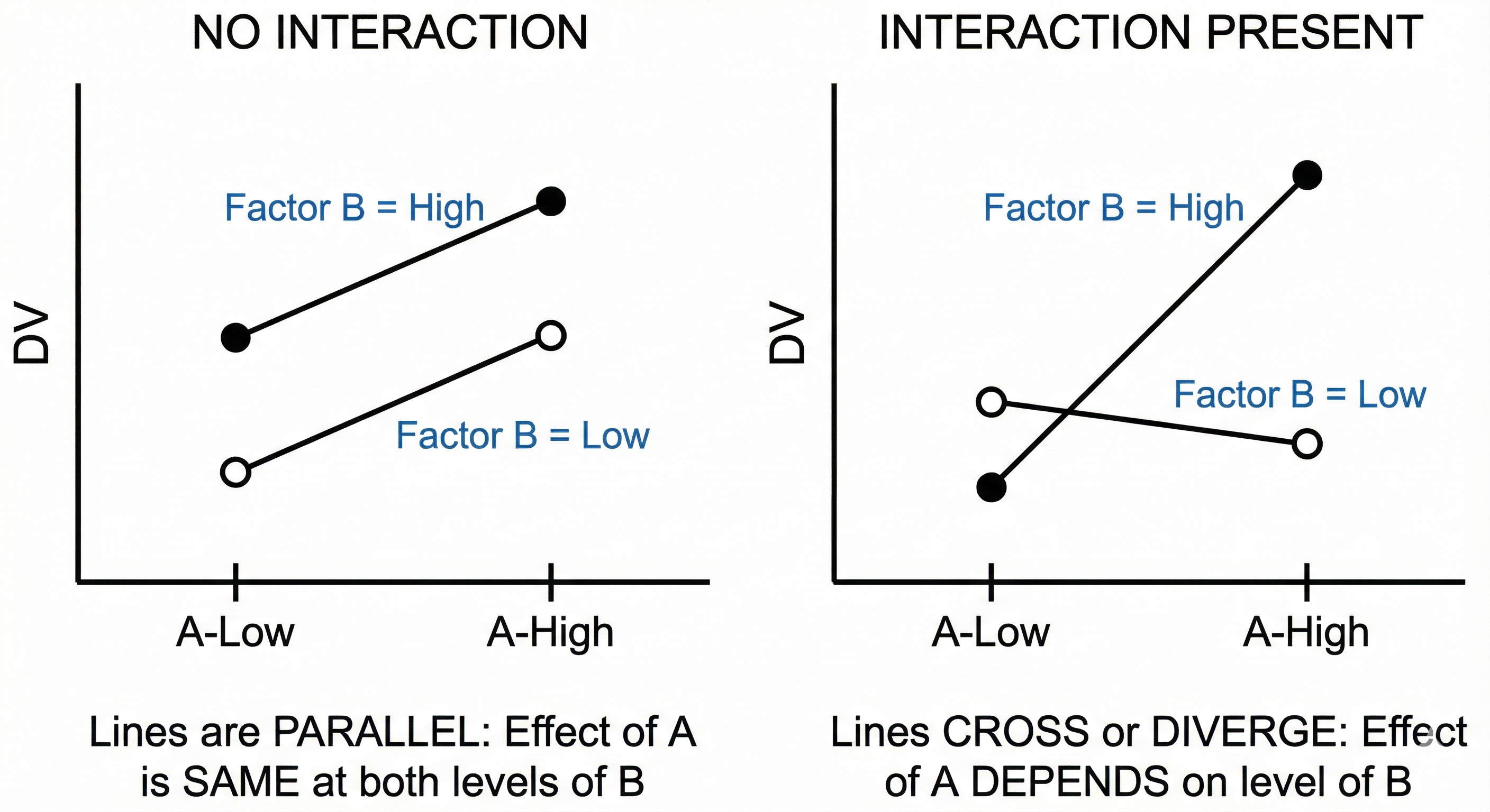
33.3. The Three Questions It Answers
- Main effect of Factor A: Does A affect the outcome, averaging across levels of B?
- Main effect of Factor B: Does B affect the outcome, averaging across levels of A?
- Interaction A×B: Does the effect of A depend on the level of B?
33.4. Understanding Interactions
33.5. Example
Research question: How do device type (phone/tablet) and user age (young/old) affect task completion time?
| Phone | Tablet | |
|---|---|---|
| Young | 45 | 40 |
| Old | 75 | 50 |
Results:
- Main effect of Device: F(1,36) = 25.3, p < .001 (tablet faster)
- Main effect of Age: F(1,36) = 42.1, p < .001 (young faster)
- Interaction Device × Age: F(1,36) = 8.7, p = .006
Interpretation: The interaction indicates that the device difference is larger for older users (25 sec) than younger users (5 sec).
33.6. ⚠️ Don't Use This When
- One or both factors have only 1 level
- Design is unbalanced and you need Type III sums of squares
- Factors are within-subjects (use repeated measures ANOVA)
33.7. Reporting Format
"A 2×2 between-subjects ANOVA revealed significant main effects of device, F(1, 36) = 25.3, p < .001, η²p = .41, and age, F(1, 36) = 42.1, p < .001, η²p = .54. These were qualified by a significant interaction, F(1, 36) = 8.7, p = .006, η²p = .19, indicating that older adults benefited more from tablets than younger adults."
34. 5.9 Repeated Measures ANOVA
34.1. What It Tests
Tests whether means differ across three or more related groups (same participants measured multiple times).
34.2. When to Use It
- Same participants measured at 3+ time points/conditions
- One continuous outcome
- Want to control for individual differences
34.3. Assumptions
- ✓ No significant outliers
- ✓ Normality of differences
- ✓ Sphericity (equal variances of differences between conditions)
34.4. The Sphericity Problem
Unlike between-subjects ANOVA, repeated measures ANOVA requires that the variances of differences between all pairs of conditions are equal.
``` Conditions: A, B, C
Sphericity requires:
Var(A-B) ≈ Var(B-C) ≈ Var(A-C)

If violated:
• F-ratio becomes too liberal (inflated Type I error)
• Use Greenhouse-Geisser or Huynh-Feldt correction
```
34.5. Example
Research question: Does performance change across three training sessions?
| Participant | Session 1 | Session 2 | Session 3 |
|---|---|---|---|
| 1 | 50 | 65 | 80 |
| 2 | 45 | 60 | 75 |
| 3 | 55 | 70 | 82 |
| 4 | 48 | 62 | 78 |
| 5 | 52 | 68 | 85 |
Mauchly's test: p = 0.12 (sphericity OK) F(2, 8) = 156.7, p < .001
Interpretation: Performance significantly improved across sessions.
34.6. ⚠️ Don't Use This When
- Only 2 conditions (use paired t-test)
- Different participants in each condition (use one-way ANOVA)
- Sphericity severely violated and corrections don't help (use MANOVA or mixed models)
34.7. Reporting Format
"A one-way repeated measures ANOVA showed a significant effect of training session on performance, F(2, 8) = 156.7, p < .001, η²p = .98. Mauchly's test indicated sphericity was met, χ²(2) = 4.27, p = .12."
35. 5.10 Kruskal-Wallis Test
35.1. What It Tests
Tests whether distributions differ across three or more independent groups. Non-parametric alternative to one-way ANOVA.
35.2. When to Use It
- 3+ independent groups
- Data is ordinal or continuous but non-normal
- Small samples with unknown distribution
35.3. Assumptions
- ✓ Independent groups
- ✓ At least ordinal data
- ✓ Similar distribution shapes (for median comparison)
35.4. The Formula
Where:
- N = total sample size
- Rⱼ = sum of ranks in group j
- nⱼ = sample size of group j
Intuition: Like ANOVA but using ranks instead of raw scores.
35.5. Example
Research question: Do three design prototypes differ in perceived usability?
| Prototype A | Prototype B | Prototype C |
|---|---|---|
| 5 | 7 | 3 |
| 4 | 8 | 2 |
| 6 | 6 | 4 |
| 3 | 7 | 3 |
H = 8.56, df = 2, p = .014
Interpretation: Usability perceptions significantly differ across prototypes.
35.6. Post-Hoc Tests
- Dunn's test with Bonferroni correction
- Mann-Whitney U tests with Bonferroni correction
35.7. ⚠️ Don't Use This When
- Data meets ANOVA assumptions (ANOVA has more power)
- Same participants across conditions (use Friedman test)
- You need to compare means specifically
35.8. Reporting Format
"A Kruskal-Wallis test indicated significant differences in usability ratings across prototypes, H(2) = 8.56, p = .014. Post-hoc Dunn's tests showed Prototype B (Mdn = 7) was rated higher than Prototype C (Mdn = 3), p = .011."
36. 5.11 Friedman Test
36.1. What It Tests
Tests whether distributions differ across three or more related groups. Non-parametric alternative to repeated measures ANOVA.
36.2. When to Use It
- Same participants measured at 3+ time points/conditions
- Data is ordinal or continuous but non-normal
- Sphericity assumption cannot be met
36.3. Assumptions
- ✓ Same participants in all conditions
- ✓ At least ordinal data
- ✓ Random sample of participants
36.4. The Formula
Where:
- n = number of participants
- k = number of conditions
- Rⱼ = sum of ranks for condition j
Process:
- Rank scores within each participant (1 to k)
- Sum ranks for each condition
- Calculate test statistic
36.5. Example
Research question: Do users rate three app interfaces differently?
| User | Interface A | Interface B | Interface C |
|---|---|---|---|
| 1 | 3 (rank 1) | 7 (rank 3) | 5 (rank 2) |
| 2 | 4 (rank 1) | 6 (rank 2) | 8 (rank 3) |
| 3 | 2 (rank 1) | 5 (rank 2) | 7 (rank 3) |
| 4 | 5 (rank 2) | 8 (rank 3) | 4 (rank 1) |
Rank sums: R_A = 5, R_B = 10, R_C = 9
χ²_F = 4.5, df = 2, p = .105
Interpretation: No significant difference in interface ratings.
36.6. Post-Hoc Tests
- Wilcoxon signed-rank tests with Bonferroni correction
- Conover test
36.7. ⚠️ Don't Use This When
- Data meets repeated measures ANOVA assumptions
- Only 2 conditions (use Wilcoxon signed-rank)
- Different participants in each group (use Kruskal-Wallis)
36.8. Reporting Format
"A Friedman test showed no significant difference in interface ratings, χ²(2) = 4.5, p = .105."
Chapter 6: Relationships Between Variables — Correlation Tests
Correlation quantifies the strength and direction of a relationship between two variables. This chapter covers when and how to use different correlation methods.
37. 6.1 Understanding Correlation Fundamentals
37.1. What Correlation Measures
Correlation coefficient (r): A standardized measure of the linear relationship between two variables.
Range: -1 to +1
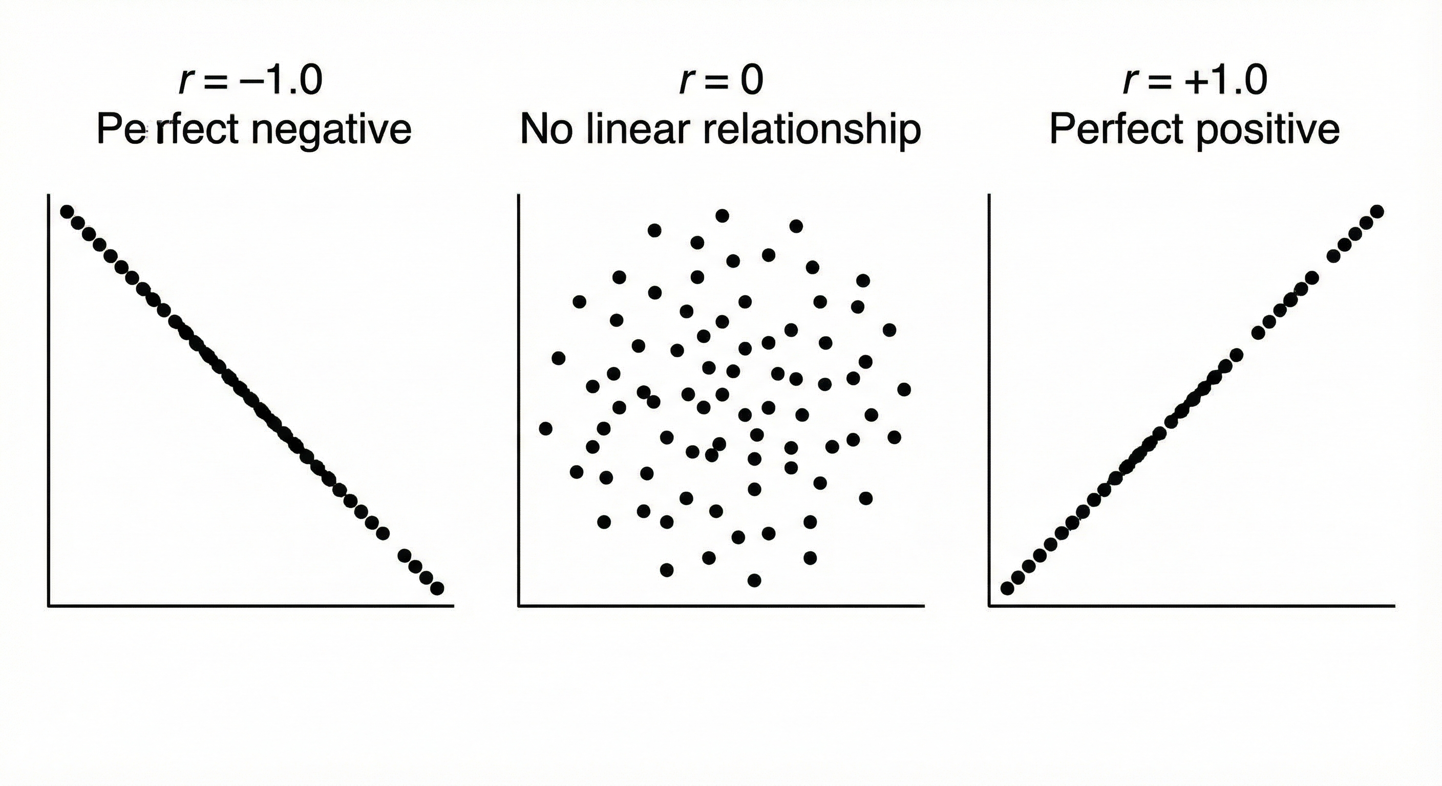
37.2. Correlation Strength Guidelines
| |r| | Interpretation | |------|----------------| | 0.00 - 0.19 | Negligible | | 0.20 - 0.39 | Weak | | 0.40 - 0.59 | Moderate | | 0.60 - 0.79 | Strong | | 0.80 - 1.00 | Very strong |
⚠️ Important: These are guidelines, not rules. Context matters! A correlation of 0.30 might be impressive in psychology but weak in physics.
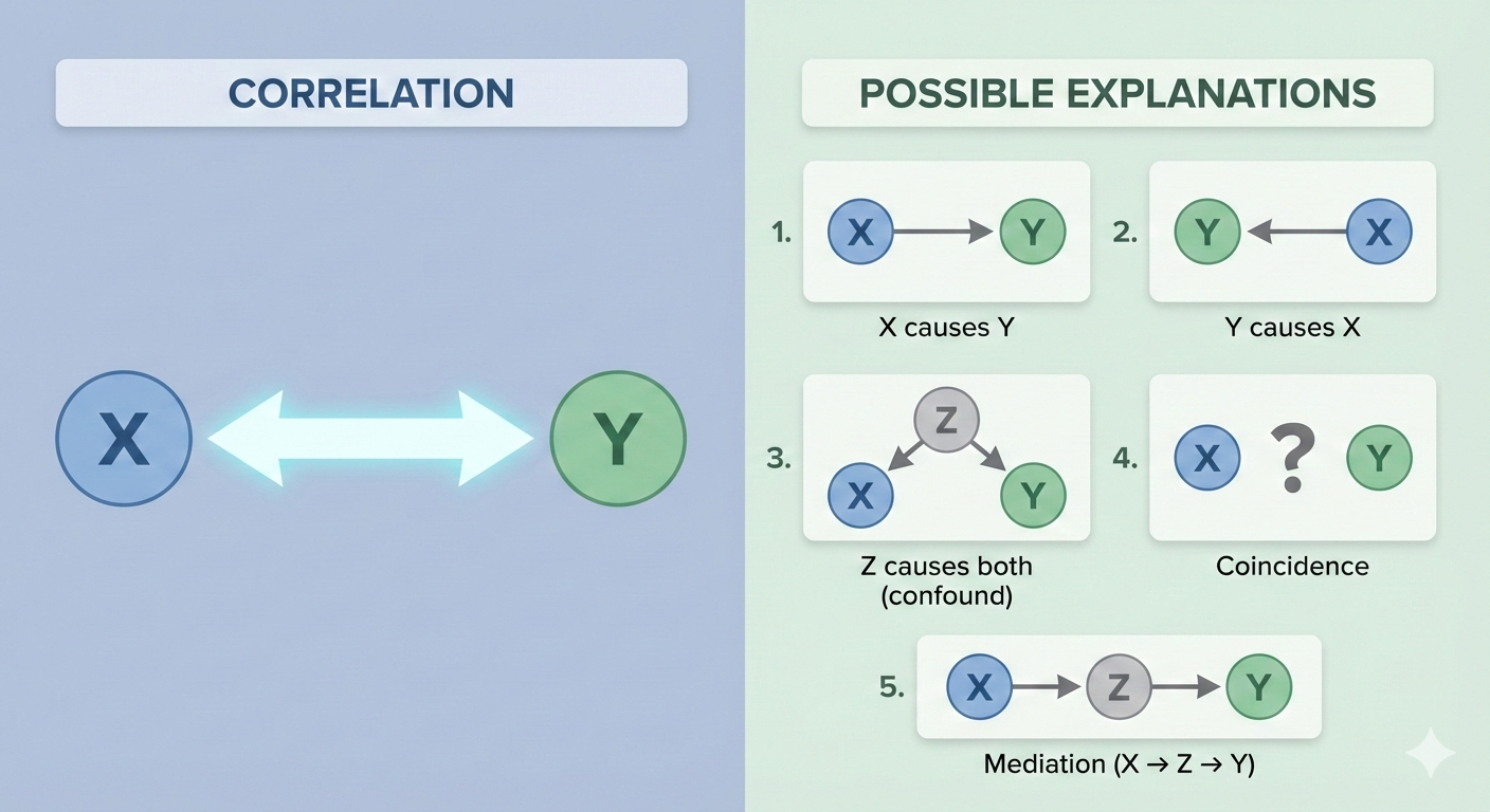
37.3. Correlation ≠ Causation
Classic examples:
- Ice cream sales and drowning deaths are correlated (both caused by hot weather)
- Shoe size and reading ability in children are correlated (both caused by age)
38. 6.2 Pearson Product-Moment Correlation
38.1. What It Tests
Measures the strength of linear relationship between two continuous variables.
38.2. When to Use It
- Both variables are continuous (interval/ratio)
- Relationship appears linear
- Both variables approximately normally distributed
- No extreme outliers
38.3. Assumptions
- ✓ Continuous data
- ✓ Linear relationship
- ✓ Bivariate normality (both variables normal)
- ✓ Homoscedasticity (equal variance across range)
- ✓ No extreme outliers
38.4. The Formula
Simplified form:
Intuition: Correlation = Covariance standardized by the product of standard deviations
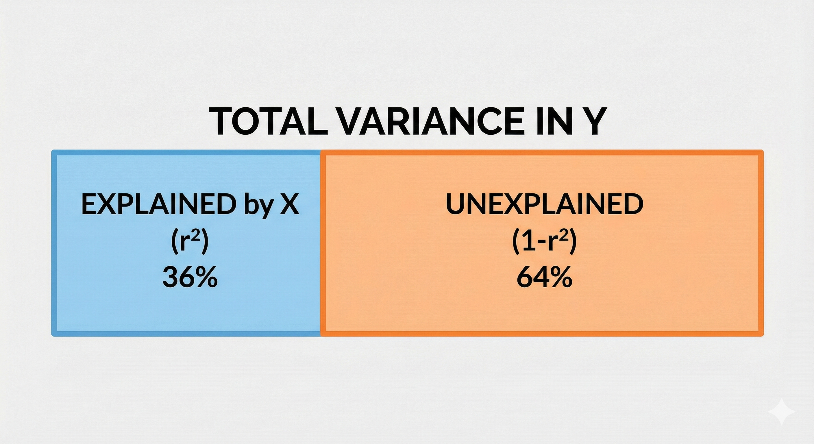
38.5. Coefficient of Determination (r²)
r² tells you the proportion of variance in Y explained by X.
If r = 0.60, then r² = 0.36 = 36% of variance explained.
38.6. ⚠️ Don't Use This When
- Relationship is non-linear (check scatter plot!)
- Data is ordinal (use Spearman)
- Severe outliers present (use Spearman)
- Non-normal distributions (use Spearman)
38.7. Reporting Format
"A Pearson correlation revealed a significant strong positive relationship between VR exposure time and motion sickness, r(4) = .97, p < .001, r² = .94."
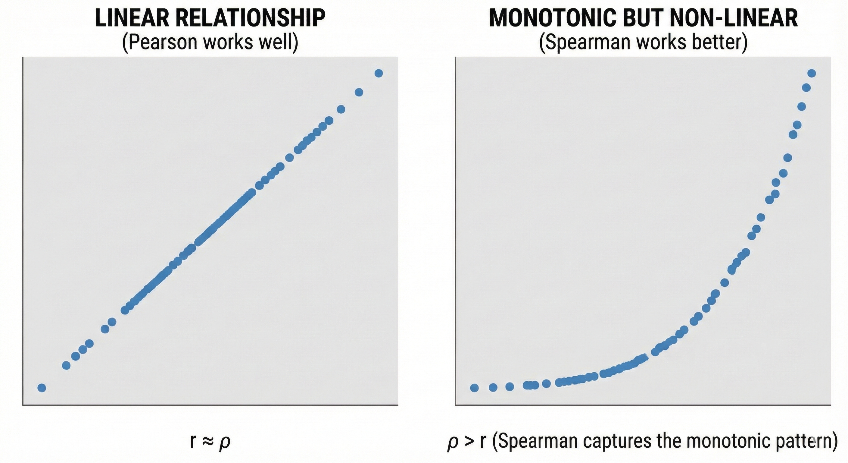
39. 6.3 Spearman Rank Correlation
39.1. What It Tests
Measures the strength of monotonic relationship between two variables using ranks.
39.2. When to Use It
- Data is ordinal
- Continuous data but non-normal
- Relationship is monotonic but not linear
- Outliers present
39.3. Assumptions
- ✓ At least ordinal data
- ✓ Monotonic relationship (consistently increasing or decreasing)
- ✓ Independent observations
39.4. The Formula
Where:
- dᵢ = difference between ranks of Xᵢ and Yᵢ
- n = number of pairs
Process:
- Rank X values (1 to n)
- Rank Y values (1 to n)
- Calculate difference between ranks for each pair
- Apply formula
39.5. When Spearman > Pearson
39.6. ⚠️ Don't Use This When
- You specifically need to measure linear relationship
- You want to quantify amount of variance explained (r² interpretation changes)
- Data is truly continuous and normal (Pearson is more powerful)
39.7. Reporting Format
"A Spearman correlation indicated a strong positive relationship between usability rankings and satisfaction rankings, ρ(3) = .80, p = .104."
40. 6.4 Other Correlation Types
40.1. Point-Biserial Correlation (rpb)
Use when: One variable is continuous, one is binary (0/1)
Example: Correlation between gender (M/F) and test scores
Note: Mathematically equivalent to Pearson correlation; gives same result.
40.2. Phi Coefficient (φ)
Use when: Both variables are binary (0/1)
Example: Correlation between purchase (yes/no) and email opened (yes/no)
Where a, b, c, d are frequencies in a 2×2 contingency table.
40.3. Kendall's Tau (τ)
Use when:
- Ordinal data with many tied ranks
- Small sample sizes
- More conservative than Spearman
40.4. Partial Correlation
Use when: You want to measure correlation between X and Y while controlling for Z.
Example: Correlation between ice cream sales and drowning, controlling for temperature.
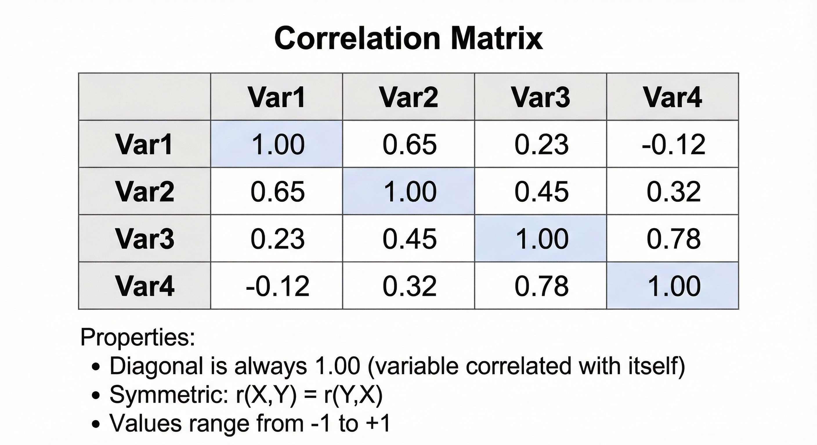
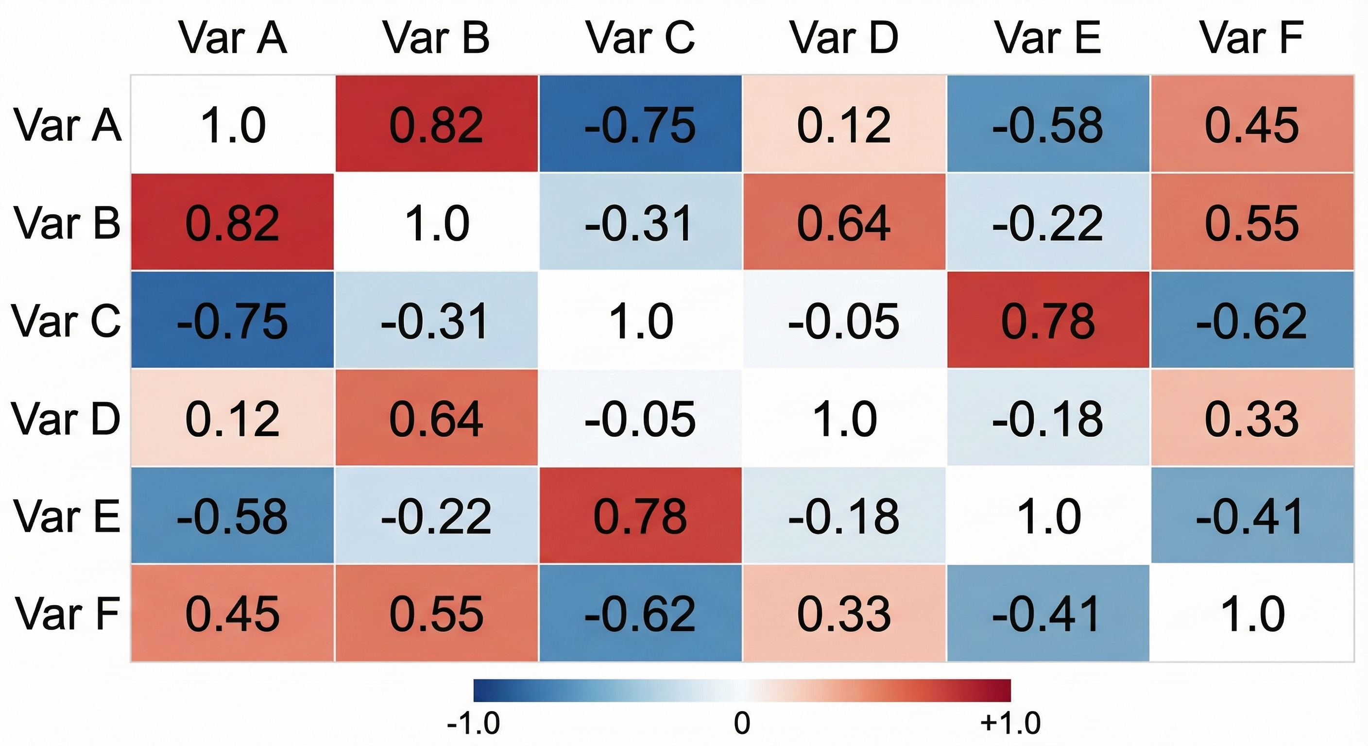
41. 6.5 The Correlation Matrix
41.1. What It Is
A table showing correlations between all pairs of variables.
41.2. Structure
41.3. When to Use It
- Exploratory data analysis
- Before regression (check for multicollinearity)
- Before factor analysis or PCA
- Identifying clusters of related variables
42. 6.6 Correlation Quick Reference
| Scenario | Test | Assumptions |
|---|---|---|
| Both continuous, linear relationship, normal | Pearson | Bivariate normality, linearity, homoscedasticity |
| One or both ordinal | Spearman | Monotonic relationship |
| Continuous but non-normal or outliers | Spearman | Monotonic relationship |
| Non-linear but monotonic | Spearman | Monotonic relationship |
| Many tied ranks, small sample | Kendall's τ | Ordinal data |
| One continuous, one binary | Point-biserial | Same as Pearson |
| Both binary | Phi (φ) | 2×2 table |
| Control for third variable | Partial correlation | Varies |
Chapter 7: Effect Size — The Forgotten Hero
P-values tell you IF an effect exists. Effect sizes tell you HOW BIG it is. This chapter explains why effect sizes matter more than p-values for practical decisions.
43. 7.1 Why Effect Size Matters
43.1. The Problem with P-Values Alone
43.2. Effect Size = Practical Significance
| Statistical Significance | Practical Significance | |
|---|---|---|
| Question | "Is there ANY effect?" | "Is the effect BIG ENOUGH to matter?" |
| Measure | p-value | Effect size |
| Influenced by | Sample size | Only the actual effect |
| Needed for | Publication conventions | Real-world decisions |
44. 7.2 Cohen's d — The Gold Standard for Mean Comparisons
44.1. What It Is
Cohen's d expresses the difference between means in standard deviation units.
44.2. The Formula
For independent groups:
Where:
For paired samples:
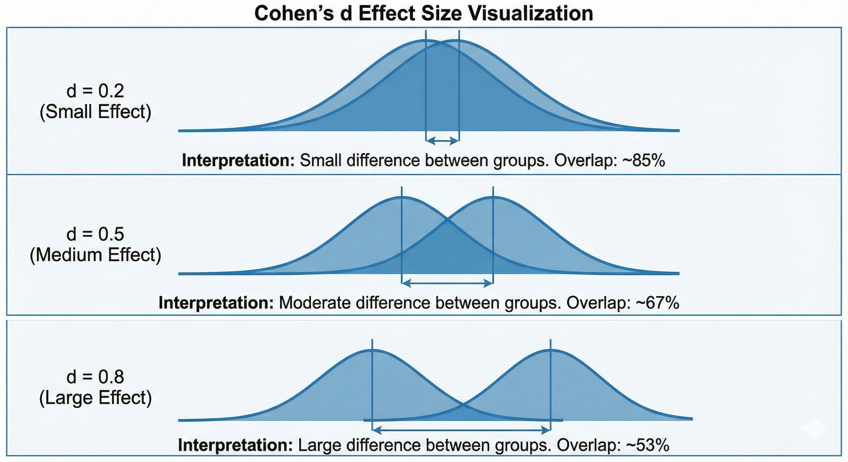
44.3. Geometric Interpretation
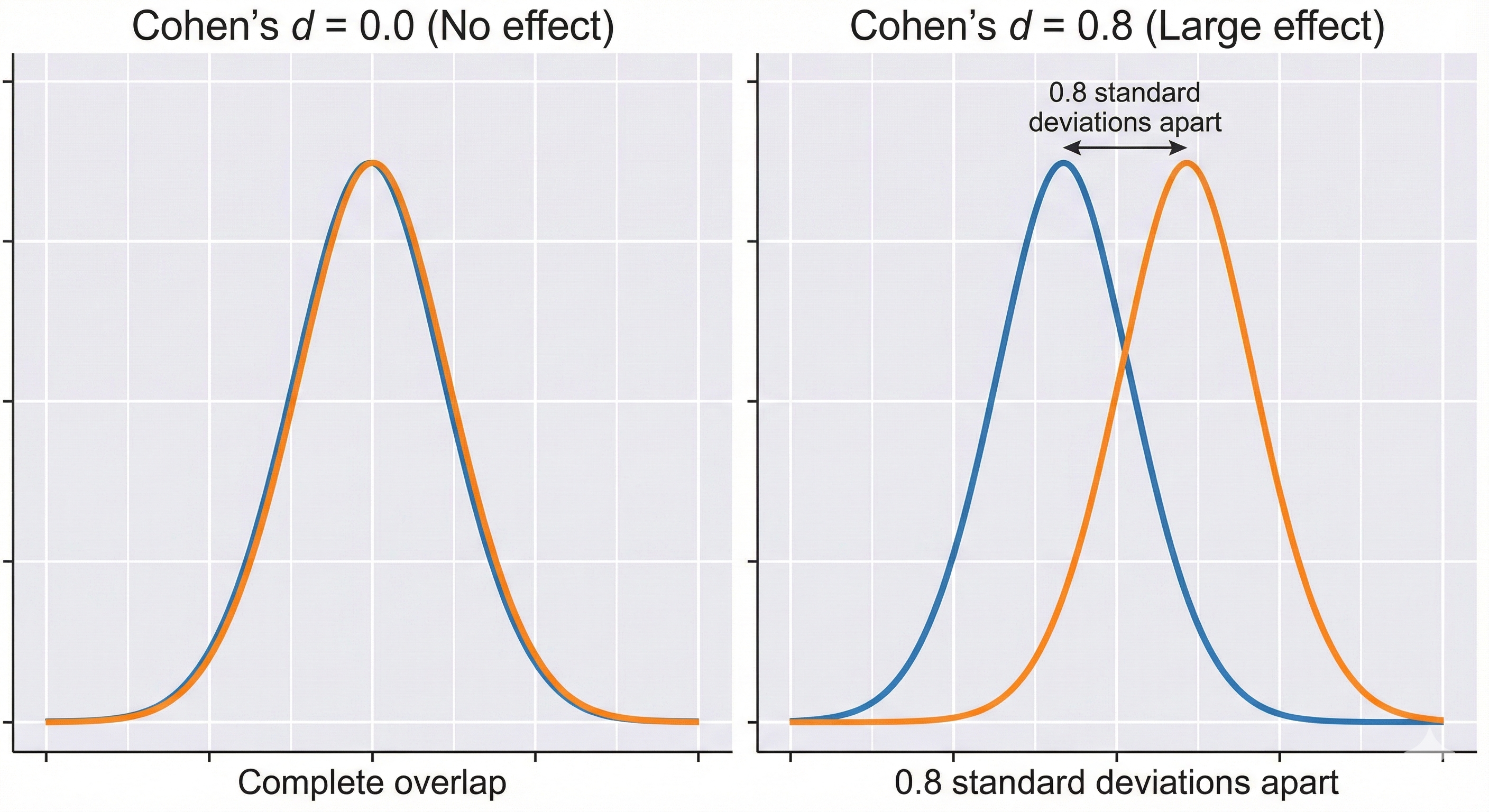
44.4. Cohen's Conventions
| d | Interpretation | Overlap |
|---|---|---|
| 0.2 | Small | 85% overlap between distributions |
| 0.5 | Medium | 67% overlap |
| 0.8 | Large | 53% overlap |
⚠️ Warning: These are guidelines, not rules! A d = 0.3 might be huge in one context and trivial in another.
45. 7.3 Eta-Squared (η²) and Partial Eta-Squared (η²p) — For ANOVA
45.1. What They Measure
Proportion of variance in the dependent variable explained by the independent variable.
45.2. Eta-Squared (η²)
Interpretation: "What proportion of total variance is due to this effect?"
45.3. Partial Eta-Squared (η²p)
Interpretation: "What proportion of variance is due to this effect, excluding variance explained by other factors?"
Use η²p when: Multiple factors in your design (two-way ANOVA, etc.)
45.4. Conventions for η² and η²p
| Value | Interpretation |
|---|---|
| 0.01 | Small |
| 0.06 | Medium |
| 0.14 | Large |
46. 7.4 Omega-Squared (ω²) — Less Biased Alternative
46.1. The Problem with η²
η² is biased—it overestimates population effect size, especially with small samples.
46.2. The Solution: Omega-Squared
Interpretation: Same as η² but less biased. Generally gives smaller (more accurate) estimates.
47. 7.5 R² — For Correlation and Regression
47.1. Coefficient of Determination
Interpretation: Proportion of variance in Y explained by X.
47.2. Example
If r = 0.60 between study hours and exam scores:
- R² = 0.36
- "Study hours explain 36% of the variance in exam scores"
47.3. Adjusted R² (For Multiple Regression)
Where k = number of predictors
Why adjusted?: Regular R² always increases when you add predictors, even useless ones. Adjusted R² penalizes for adding non-helpful predictors.
48. 7.6 r (Effect Size for Non-Parametric Tests)
48.1. Converting to r
For non-parametric tests, convert test statistics to r:
From Mann-Whitney U:
From Wilcoxon:
48.2. Conventions for r as Effect Size
| r | Interpretation |
|---|---|
| 0.10 | Small |
| 0.30 | Medium |
| 0.50 | Large |
49. 7.7 Odds Ratio (OR) and Relative Risk (RR)
49.1. For Categorical Outcomes
Odds Ratio:
Using a 2×2 table:
| Outcome + | Outcome - | |
|---|---|---|
| Group 1 | a | b |
| Group 2 | c | d |
Interpretation:
- OR = 1: No difference
- OR > 1: Outcome more likely in Group 1
- OR < 1: Outcome less likely in Group 1
50. 7.8 Effect Size Quick Reference
| Test Type | Effect Size Measure | Small | Medium | Large |
|---|---|---|---|---|
| t-tests | Cohen's d | 0.2 | 0.5 | 0.8 |
| ANOVA | η² or η²p | 0.01 | 0.06 | 0.14 |
| ANOVA (unbiased) | ω² | 0.01 | 0.06 | 0.14 |
| Correlation | r or R² | 0.1 / 0.01 | 0.3 / 0.09 | 0.5 / 0.25 |
| Chi-square | Cramér's V | 0.1 | 0.3 | 0.5 |
| Non-parametric | r | 0.1 | 0.3 | 0.5 |
51. 7.9 Coefficient of Variation (CV)
51.1. What It Is
The coefficient of variation expresses standard deviation as a percentage of the mean.
51.2. When to Use It
- Comparing variability between datasets with different units
- Comparing variability between datasets with different means
- Assessing measurement precision
- Quality control
51.3. Example
Comparing consistency of two instruments:
- Instrument A: M = 100, SD = 5 → CV = 5%
- Instrument B: M = 1000, SD = 30 → CV = 3%
Instrument B is more consistent despite having larger SD!
51.4. Limitations
- Meaningless when mean is close to zero
- Requires ratio-scale data (true zero point)
Chapter 8: Categorical Data Analysis
When your data is counts or categories rather than measurements, you need different tests.
52. 8.1 Chi-Square Goodness-of-Fit Test
52.1. What It Tests
Tests whether observed frequencies match expected frequencies for a single categorical variable.
52.2. When to Use It
- One categorical variable
- Testing if distribution matches expectation
- Expected frequencies ≥ 5 in each category
52.3. The Formula
Where:
- Oᵢ = observed frequency in category i
- Eᵢ = expected frequency in category i
Intuition: Sum up standardized squared deviations from expectation.
52.4. Degrees of Freedom
df = k - 1 (where k = number of categories)
52.5. Example
Research question: Do users prefer certain color schemes equally?
| Color | Observed | Expected (equal preference) |
|---|---|---|
| Blue | 45 | 30 |
| Green | 28 | 30 |
| Red | 17 | 30 |
| Total | 90 | 90 |
df = 3 - 1 = 2, p < .01
Interpretation: Color preferences are not equal; blue is preferred.
52.6. ⚠️ Don't Use This When
- Any expected frequency < 5 (use exact tests or combine categories)
- Data is continuous (use different test)
- Two categorical variables (use chi-square test of independence)
52.7. Reporting Format
"A chi-square goodness-of-fit test indicated that color preferences were not equally distributed, χ²(2) = 13.27, p = .001."
53. 8.2 Chi-Square Test of Independence
53.1. What It Tests
Tests whether two categorical variables are related (associated).
53.2. When to Use It
- Two categorical variables
- Independent observations
- Expected frequencies ≥ 5 in most cells
53.3. The Formula
Where expected frequency:
53.4. Degrees of Freedom
df = (rows - 1) × (columns - 1)
53.5. Example
Research question: Is there an association between device type and task completion?
| Completed | Not Completed | Total | |
|---|---|---|---|
| Phone | 40 | 20 | 60 |
| Tablet | 55 | 5 | 60 |
| Total | 95 | 25 | 120 |
χ² = 11.37, df = 1, p < .001
Interpretation: Device type and task completion are significantly associated.
53.6. Effect Size: Cramér's V
Where k = min(rows, columns)
V ranges from 0 (no association) to 1 (perfect association).
53.7. ⚠️ Don't Use This When
- Expected values < 5 in more than 20% of cells (use Fisher's exact)
- 2×2 table with small N (use Fisher's exact)
- Paired/repeated observations (use McNemar)
53.8. Reporting Format
"A chi-square test of independence showed a significant association between device type and task completion, χ²(1) = 11.37, p < .001, V = .31."
54. 8.3 Fisher's Exact Test
54.1. What It Tests
Same as chi-square test of independence, but exact (no approximation).
54.2. When to Use It
- 2×2 contingency table
- Small sample (N < 20)
- Expected frequencies < 5
54.3. How It Works
Calculates the exact probability of obtaining the observed (or more extreme) table, given fixed marginal totals.
54.4. ⚠️ Don't Use This When
- Large samples (chi-square is fine and faster)
- Tables larger than 2×2 with large N
54.5. Reporting Format
"Fisher's exact test revealed a significant association between tutorial use and configuration success, p = .047, OR = 11.67."
55. 8.4 McNemar's Test
55.1. What It Tests
Tests for changes in proportions when the same subjects are measured twice (paired categorical data).
55.2. When to Use It
- Same subjects measured before and after
- Binary outcome (yes/no)
- Interested in whether proportions changed
55.3. The Setup
| After: Yes | After: No | |
|---|---|---|
| Before: Yes | a | b |
| Before: No | c | d |
55.4. The Formula
Intuition: Only cells b and c matter (people who changed). Tests if changers were equally likely to go in either direction.
55.5. Example
Research question: Did training change whether employees follow safety protocols?
| After: Follow | After: Don't Follow | |
|---|---|---|
| Before: Follow | 45 | 5 |
| Before: Don't Follow | 20 | 10 |
df = 1, p = .003
Interpretation: The training significantly changed behavior.
55.6. ⚠️ Don't Use This When
- Observations are independent (use chi-square)
- More than 2 categories (use Cochran's Q or Bowker's test)
- b + c < 25 (use exact McNemar test)
55.7. Reporting Format
"McNemar's test indicated a significant change in protocol adherence after training, χ²(1) = 9.0, p = .003."
56. 8.5 Cochran's Q Test
56.1. What It Tests
Extension of McNemar's test for three or more related groups with binary outcomes.
56.2. When to Use It
- Same subjects measured at 3+ time points
- Binary outcome
- Repeated measures design
56.3. Reporting Format
"Cochran's Q test showed significant differences in preference across design iterations, Q(2) = 12.5, p = .002."
Chapter 9: Advanced Techniques
This chapter briefly covers techniques for complex data structures.
57. 9.1 Principal Component Analysis (PCA)
57.1. What It Does
Reduces many correlated variables to fewer uncorrelated components.
57.2. When to Use It
- Too many variables to analyze individually
- Variables are correlated (redundant)
- Want to identify underlying dimensions
- Data preprocessing for other analyses
57.3. How It Works (Conceptual)
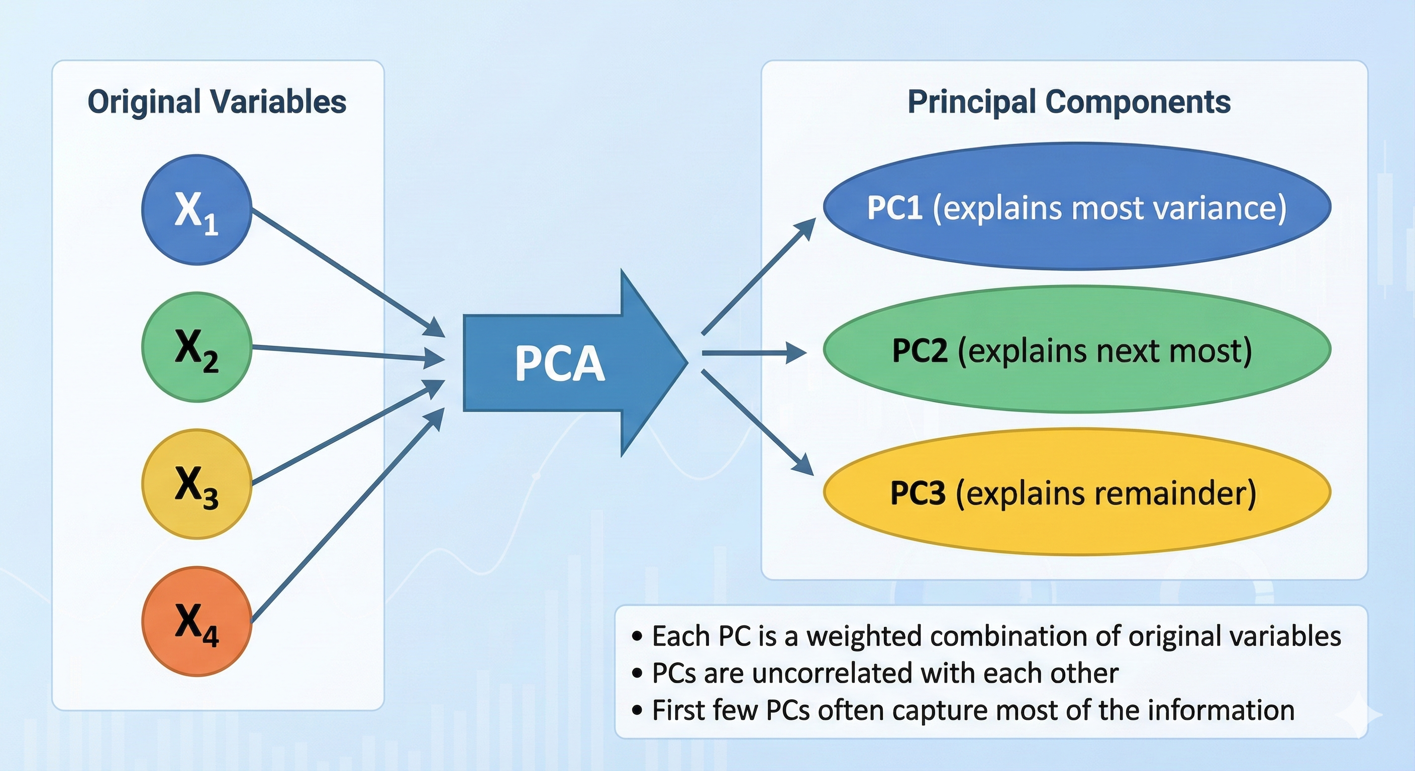
57.4. Key Outputs
- Eigenvalues: Variance explained by each component
- Eigenvectors: Weights defining each component
- Loadings: Correlations between variables and components
- Scores: Values of components for each observation
57.5. Deciding How Many Components to Keep
| Method | Rule |
|---|---|
| Kaiser criterion | Keep components with eigenvalue > 1 |
| Scree plot | Keep components before the "elbow" |
| Variance explained | Keep enough to explain 70-80% |
57.6. Assumptions
- Continuous or at least interval data
- Linear relationships between variables
- Adequate sample size (n > 5 per variable, ideally)
- Sufficient correlations (KMO > 0.6, Bartlett's test significant)
57.7. ⚠️ Don't Use This When
- Variables are clearly independent (nothing to reduce)
- You need interpretable factors (consider Factor Analysis)
- Data is categorical (use Multiple Correspondence Analysis)
58. 9.2 Factor Analysis
58.1. What It Does
Identifies latent (hidden) factors that explain correlations among variables.
58.2. Difference from PCA
| PCA | Factor Analysis |
|---|---|
| Data reduction technique | Theory-driven model |
| Components are exact mathematical constructs | Factors are assumed to cause observed correlations |
| Explains all variance | Explains only shared variance (communality) |
| No assumptions about underlying structure | Assumes latent factors exist |
58.3. When to Use It
- Developing or validating a questionnaire
- Testing theoretical constructs
- Identifying dimensions of a concept
59. 9.3 Mixed-Effects Models (Brief Overview)
59.1. What They Do
Handle data with both fixed effects (your experimental variables) and random effects (grouping structures like participants or items).
59.2. When to Use Them
- Repeated measures with missing data
- Nested data (students within schools)
- Crossed random effects (participants × items)
- Unbalanced designs
59.3. Why They're Increasingly Preferred
- More flexible than traditional ANOVA
- Handle missing data gracefully
- Don't require sphericity
- Model individual differences
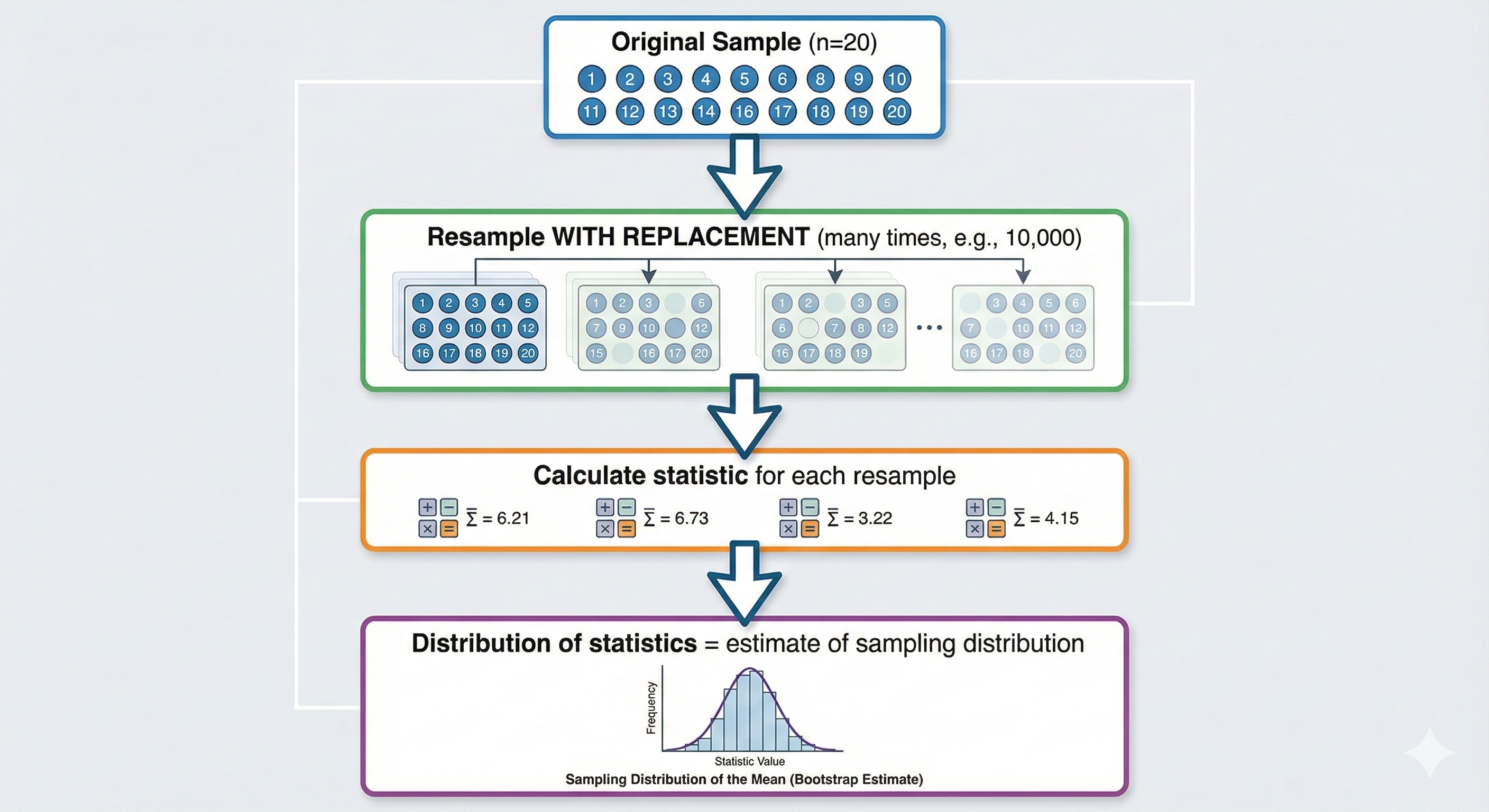
60. 9.4 Bootstrap Methods (Brief Overview)
60.1. What They Do
Estimate sampling distributions by repeatedly resampling from your data.
60.2. When to Use Them
- Assumptions of parametric tests are violated
- Calculating confidence intervals for complex statistics
- Small samples where distribution is unclear
60.3. Basic Concept
Chapter 10: Bayesian Alternatives — The Other Paradigm
This chapter provides a brief introduction to Bayesian approaches as alternatives to the frequentist tests covered earlier.
61. 10.1 Key Differences Revisited
61.1. Frequentist vs. Bayesian
| Aspect | Frequentist | Bayesian |
|---|---|---|
| Probability means | Long-run frequency | Degree of belief |
| Parameters are | Fixed but unknown | Random variables with distributions |
| Data is | Random | Fixed (observed) |
| Question asked | P(data | hypothesis) | P(hypothesis | data) |
| Result | P-value, confidence interval | Posterior distribution, credible interval |
| Prior information | Not used formally | Explicitly included |
62. 10.2 Bayesian Equivalents of Common Tests
| Frequentist Test | Bayesian Equivalent |
|---|---|
| One-sample t-test | Bayesian one-sample test |
| Independent t-test | Bayesian independent samples test |
| Paired t-test | Bayesian paired samples test |
| ANOVA | Bayesian ANOVA |
| Correlation | Bayesian correlation |
| Chi-square | Bayesian contingency table analysis |
62.1. Bayes Factor (BF)
The Bayesian equivalent of hypothesis testing uses the Bayes Factor:
Interpretation:
| BF₁₀ | Evidence for H₁ |
|---|---|
| 1-3 | Anecdotal |
| 3-10 | Moderate |
| 10-30 | Strong |
| 30-100 | Very strong |
| >100 | Extreme |
Key advantage: BF can provide evidence FOR the null hypothesis (BF < 1), not just fail to reject it!
62.2. Credible Intervals vs. Confidence Intervals
95% Confidence Interval (frequentist): "If we repeated this study infinitely, 95% of calculated intervals would contain the true parameter."
95% Credible Interval (Bayesian): "Given the data and prior, there's a 95% probability the parameter lies in this interval."
The Bayesian interpretation is what most people think confidence intervals mean!
63. 10.3 When to Consider Bayesian Methods
Advantages:
- Intuitive probability statements
- Can provide evidence for null hypothesis
- Incorporates prior knowledge
- No p-value problems (p-hacking, misinterpretation)
Challenges:
- Requires specifying priors (can be controversial)
- Computationally intensive
- Less familiar to reviewers
- Software learning curve
64. 10.4 Reporting Bayesian Results
"A Bayesian independent samples t-test revealed strong evidence for a difference between groups, BF₁₀ = 24.3. The posterior distribution of the effect size had a median of 0.72 (95% CI [0.35, 1.12])."
Chapter 11: Statistical Sins Researchers Commit
This chapter covers common mistakes that lead to incorrect conclusions. Learn from others' errors!
65. 11.1 P-Hacking: The Garden of Forking Paths
65.1. What It Is
Manipulating analysis (consciously or unconsciously) to achieve p < 0.05.
65.2. Common P-Hacking Techniques
| Sin | Description |
|---|---|
| Selective reporting | Only reporting significant results |
| Optional stopping | Stopping data collection when p < 0.05 |
| Outcome switching | Changing primary outcome to one that's significant |
| Covariate fishing | Adding/removing covariates until significant |
| Subgroup searching | Testing many subgroups, reporting significant ones |
| Multiple testing | Running many tests, reporting without correction |
65.3. Real Example
A famous simulation showed that through various "researcher degrees of freedom," you could find "significant" effects for almost anything—including demonstrating that listening to certain songs makes people younger!
65.4. Prevention
- Pre-register your analysis plan
- Report all analyses conducted
- Use correction for multiple comparisons
- Distinguish exploratory from confirmatory

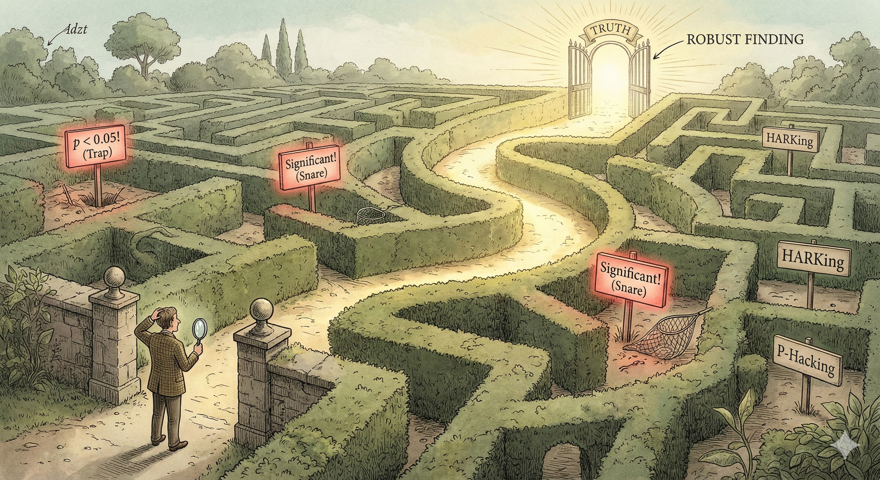
66. 11.2 HARKing: Hypothesizing After Results are Known
66.1. What It Is
Presenting exploratory findings as if they were predicted all along.
66.2. Why It's a Problem
- Inflates false positive rate
- Makes findings seem more credible than warranted
- Prevents accurate assessment of evidence
66.3. Real Example
"We hypothesized that effect X would occur in subgroup Y" — when actually you tested 20 subgroups and only reported the one significant finding.
66.4. Prevention
- Pre-register hypotheses before data collection
- Clearly label exploratory analyses
- Be honest about the discovery process
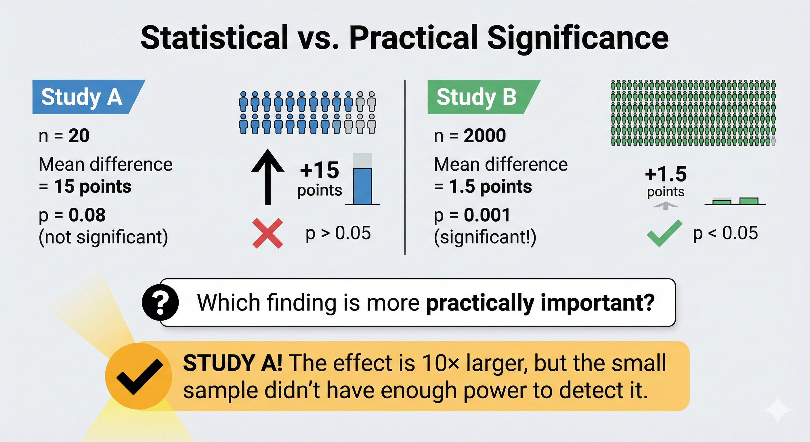
67. 11.3 Confusing Statistical and Practical Significance
67.1. The Problem
Statistical significance (p < 0.05) only means the effect is unlikely to be exactly zero.
Practical significance means the effect is large enough to matter.
67.2. Real Example
A study with n = 100,000 found that a new teaching method improved test scores by 0.1 points (out of 100), p < 0.001.
Statistically significant? Yes! Practically significant? Absolutely not!
67.3. Prevention
- Always report and interpret effect sizes
- Calculate confidence intervals around effect sizes
- Ask: "Would this effect change any decisions?"
68. 11.4 Violating Independence Assumptions
68.1. The Problem
Using tests that assume independence when observations are not independent.
68.2. Common Violations
| Situation | Problem | Solution |
|---|---|---|
| Students in classrooms | Students in same class are correlated | Mixed-effects models |
| Repeated measures treated as independent | Same person's data points are correlated | Repeated measures ANOVA |
| Time series data | Adjacent time points are correlated | Time series analysis |
68.3. Real Example
Testing whether a teaching intervention worked by treating each quiz score as independent, when actually the same 30 students took 10 quizzes each (n = 300 is actually n = 30!).
69. 11.5 Post-Hoc Power Analysis
69.1. The Problem
Calculating power AFTER finding a non-significant result to argue "we just needed more participants."
69.2. Why It's Meaningless
Post-hoc power is mathematically determined by the p-value. If p = 0.05, post-hoc power ≈ 50%. Always. The calculation adds no new information.
69.3. What To Do Instead
- Report effect sizes and confidence intervals
- Acknowledge limitations of sample size
- Plan power analysis BEFORE data collection
70. 11.6 Dichotomizing Continuous Variables
70.1. The Problem
Splitting continuous variables into high/low groups (e.g., median split).
70.2. Why It's Bad
- Throws away information
- Reduces statistical power
- Can create spurious effects
- Treats "just above median" and "far above median" as identical
70.3. Real Example
Splitting participants into "high anxiety" and "low anxiety" based on median score, then comparing groups. Someone who scored 49 (low) is treated as fundamentally different from someone who scored 51 (high), even though they're essentially the same.
70.4. What To Do Instead
- Keep variables continuous when possible
- Use regression instead of group comparisons
- If you must categorize, use established clinical cutoffs
71. 11.7 Ignoring Multiple Comparisons
71.1. The Problem
Running many tests without correcting for inflated false positive rate.
71.2. The Math
If you run 20 tests at α = 0.05:
- Probability of at least one false positive = 1 - (0.95)²⁰ = 64%!
71.3. Correction Methods
| Method | Approach | Use When |
|---|---|---|
| Bonferroni | Divide α by number of tests | Conservative, few tests |
| Holm-Bonferroni | Sequential rejection procedure | Better power than Bonferroni |
| False Discovery Rate (FDR) | Control proportion of false discoveries | Many tests (genomics, neuroimaging) |
| Tukey HSD | Designed for pairwise comparisons after ANOVA | ANOVA post-hoc |
71.4. Real Example
A researcher tested 100 brain regions for activity differences and reported the 5 "significant" findings. Without correction, ~5 false positives are expected by chance!
72. 11.8 Misinterpreting Non-Significant Results
72.1. The Problem
Claiming "no effect" or "no difference" when p > 0.05.
72.2. The Reality
Non-significance means:
- "We don't have enough evidence to reject the null"
- NOT "The null hypothesis is true"
- NOT "There is no effect"
72.3. What Affects Power to Detect Effects
- Sample size (too small?)
- Effect size (too small to detect?)
- Variance (too noisy?)
- Measurement (too imprecise?)
72.4. What To Do Instead
- Report effect sizes and confidence intervals
- Discuss power limitations
- Consider equivalence testing (TOST) to actually support "no difference"
- Use Bayesian methods to quantify evidence for null
73. 11.9 The Sin Summary Checklist
Before submitting your paper, check:
| Sin | Check | |
|---|---|---|
| □ | P-hacking | Did I pre-register? Did I report all analyses? |
| □ | HARKing | Am I honestly distinguishing confirmatory from exploratory? |
| □ | Significance confusion | Did I report and interpret effect sizes? |
| □ | Independence violation | Are my observations truly independent? |
| □ | Post-hoc power | Did I avoid this meaningless calculation? |
| □ | Dichotomization | Did I keep continuous variables continuous? |
| □ | Multiple comparisons | Did I correct for multiple tests? |
| □ | Non-significance claims | Did I avoid claiming "no effect" from p > 0.05? |
Chapter 12: Quick Reference & Cheat Sheets
74. 12.1 Test Selection Cheat Sheet
74.1. By Research Question
| Research Question | Parametric Test | Non-Parametric Alternative |
|---|---|---|
| Is sample mean different from known value? | One-sample t-test | Wilcoxon signed-rank (one-sample) |
| Do two independent groups differ? | Independent t-test | Mann-Whitney U |
| Do paired observations differ? | Paired t-test | Wilcoxon signed-rank |
| Do 3+ independent groups differ? | One-way ANOVA | Kruskal-Wallis |
| Do 3+ related conditions differ? | Repeated measures ANOVA | Friedman test |
| Are two continuous variables related? | Pearson correlation | Spearman correlation |
| Are two categorical variables related? | Chi-square test | Fisher's exact test |
| Did proportions change (paired binary)? | — | McNemar's test |
74.2. By Data Type
| DV Type | IV Type | Groups | Parametric | Non-Parametric |
|---|---|---|---|---|
| Continuous | — | 1 vs. value | One-sample t | Wilcoxon (1-samp) |
| Continuous | Categorical | 2 independent | Independent t | Mann-Whitney U |
| Continuous | Categorical | 2 paired | Paired t | Wilcoxon signed |
| Continuous | Categorical | 3+ independent | One-way ANOVA | Kruskal-Wallis |
| Continuous | Categorical | 3+ paired | RM ANOVA | Friedman |
| Continuous | Continuous | — | Pearson r | Spearman ρ |
| Categorical | Categorical | Independent | Chi-square | Fisher's exact |
| Binary | Before/After | Paired | — | McNemar |
75. 12.2 Assumption Checking Cheat Sheet
| Assumption | How to Check | What If Violated? |
|---|---|---|
| Normality | Shapiro-Wilk test, Q-Q plot | Use non-parametric or transform |
| Homogeneity of variance | Levene's test | Use Welch's correction |
| Sphericity | Mauchly's test | Use G-G or H-F correction |
| Independence | Study design | Use appropriate repeated measures test |
| Linearity | Scatter plot | Use Spearman or transform |
| No extreme outliers | Boxplots, Z-scores > 3 | Remove/Winsorize or use robust methods |
76. 12.3 Effect Size Cheat Sheet
| Test | Effect Size | Small | Medium | Large |
|---|---|---|---|---|
| t-tests | Cohen's d | 0.2 | 0.5 | 0.8 |
| ANOVA | η² or η²p | 0.01 | 0.06 | 0.14 |
| Correlation | r | 0.1 | 0.3 | 0.5 |
| Chi-square | Cramér's V | 0.1 | 0.3 | 0.5 |
| Non-parametric | r (from Z) | 0.1 | 0.3 | 0.5 |
77. 12.4 Reporting Statistics Cheat Sheet
77.1. Format Template
| Test | Report Format |
|---|---|
| t-test | t(df) = X.XX, p = .XXX, d = X.XX |
| ANOVA | F(df₁, df₂) = X.XX, p = .XXX, η²p = .XX |
| Chi-square | χ²(df) = X.XX, p = .XXX, V = .XX |
| Correlation | r(df) = .XX, p = .XXX |
| Mann-Whitney | U = XXX, p = .XXX, r = .XX |
| Wilcoxon | W = XXX, p = .XXX, r = .XX |
| Kruskal-Wallis | H(df) = X.XX, p = .XXX |
| Friedman | χ²(df) = X.XX, p = .XXX |
77.2. Rules
- Report exact p-values (p = .023), not just p < .05
- Round to 2-3 decimal places
- Always include effect size
- Include degrees of freedom
- Report means and SDs for described groups
78. 12.5 Distribution Quick Reference
| Distribution | Shape | Parameters | Use For |
|---|---|---|---|
| Normal | Symmetric bell | μ (mean), σ (SD) | Continuous measurements |
| t | Bell with heavy tails | df | Small sample means |
| Chi-square | Right-skewed | df | Categorical tests |
| F | Right-skewed | df₁, df₂ | Variance ratios (ANOVA) |
| Binomial | Discrete, symmetric-ish | n, p | Count of successes |
| Poisson | Discrete, right-skewed | λ | Event counts |
79. 12.6 Critical Values Quick Reference
79.1. t-Distribution (Two-Tailed, α = 0.05)
| df | Critical t |
|---|---|
| 5 | 2.571 |
| 10 | 2.228 |
| 15 | 2.131 |
| 20 | 2.086 |
| 30 | 2.042 |
| 60 | 2.000 |
| 120 | 1.980 |
| ∞ | 1.960 |
79.2. Chi-Square (α = 0.05)
| df | Critical χ² |
|---|---|
| 1 | 3.841 |
| 2 | 5.991 |
| 3 | 7.815 |
| 4 | 9.488 |
| 5 | 11.070 |
80. 12.7 Sample Size Rules of Thumb
| Test | Minimum per Group | Recommended |
|---|---|---|
| t-test | 12 | 20-30 |
| ANOVA | 12 | 20 |
| Correlation | 20 | 50+ |
| Chi-square | Expected ≥ 5 | 20+ per cell |
| Regression | 10-15 per predictor | 20 per predictor |
| Factor analysis | 5 per variable | 10+ per variable |
Note: These are minimums. Always do a proper power analysis for your specific situation!
81. 12.8 Decision Tree Summary (All-in-One)
82. 12.9 Master Formula Sheet
82.1. Descriptive Statistics
82.2. Test Statistics
82.3. Effect Sizes
Conclusion: The Path Forward
You've now traversed the landscape of statistical testing. Here's what to remember:
-
Always start with your research question — What are you trying to learn?
-
Know your data — What type? What distribution? What assumptions can you make?
-
Use the decision trees — Don't memorize; navigate.
-
Check assumptions first — Before running any parametric test.
-
Report effect sizes — P-values alone are not enough.
-
Avoid the statistical sins — Pre-register, report everything, don't p-hack.
-
When in doubt, use non-parametric — They're more robust, just less powerful.
-
Consider Bayesian alternatives — Especially when you want to support the null.
Statistics is not about finding "significance" — it's about quantifying evidence to answer meaningful questions. The best analysis is one that honestly addresses your research question, acknowledges its limitations, and guides future inquiry.
Good luck with your research!
*Last updated: Jan 2026
This guide is provided for educational purposes. Always consult with a statistician for complex analyses or when stakes are high.
Appendix A: Glossary of Terms
| Term | Definition |
|---|---|
| α (alpha) | Significance level; probability of Type I error |
| β (beta) | Probability of Type II error |
| Confidence Interval | Range likely to contain population parameter |
| Degrees of Freedom (df) | Number of independent values that can vary |
| Effect Size | Magnitude of an effect, independent of sample size |
| H₀ (null hypothesis) | Statement of no effect/difference |
| H₁ (alternative hypothesis) | Statement that there is an effect/difference |
| Homogeneity of variance | Equal variances across groups |
| Non-parametric | Tests that don't assume specific distributions |
| Normal distribution | Symmetric bell-shaped distribution |
| p-value | Probability of results this extreme if H₀ is true |
| Parametric | Tests that assume specific distributions |
| Power | Probability of correctly rejecting a false H₀ |
| Sphericity | Equal variances of differences (repeated measures) |
| Type I Error | False positive (rejecting true H₀) |
| Type II Error | False negative (failing to reject false H₀) |
Appendix B: Recommended Reading
Introductory:
- Field, A. - Discovering Statistics Using IBM SPSS Statistics
- Navarro, D. - Learning Statistics with R (free online)
Intermediate:
- Cohen, J. - Statistical Power Analysis for the Behavioral Sciences
- Cumming, G. - Understanding the New Statistics
Advanced:
- Gelman, A. & Hill, J. - Data Analysis Using Regression and Multilevel/Hierarchical Models
- McElreath, R. - Statistical Rethinking (Bayesian)
End of Guide
Thank you for reading. May your p-values be meaningful and your effect sizes be large!